https://doi.org/10.5194/amt-10-3265-2017 © Author(s) 2017. This work is distributed under the Creative Commons Attribution 3.0 License.
Mean wind vector estimation using the velocity–azimuth display
(VAD) method: an explicit algebraic solution
Gerd Teschke1and Volker Lehmann2
1Institute for Computational Mathematics in Science and Technology, University of Applied Sciences Neubrandenburg, Brodaer Str. 2, 17033 Neubrandenburg, Germany
2Deutscher Wetterdienst, Meteorologisches Observatorium Lindenberg, Am Observatorium 12, 15848 Tauche-Lindenberg, Germany
Correspondence to:Gerd Teschke ([email protected])
Received: 3 November 2016 – Discussion started: 20 January 2017
Revised: 18 May 2017 – Accepted: 11 July 2017 – Published: 6 September 2017
Abstract. This paper deals with the analysis of the sam-pling setup for Doppler profilers aiming at the determina-tion of vertical profiles of the wind. An explicit soludetermina-tion for the retrieval of mean wind vectors under the assumption of local homogeneity is presented for the case of a symmetric velocity–azimuth display sampling, and a stability analysis is performed. Furthermore, the explicit solution allows a de-tailed investigation of the propagation of radial wind mea-surement errors on the retrieved wind vector.
1 Introduction
The wind vector is a fundamental variable for describing the state of the atmosphere (Dutton, 1986); it can be measured with a variety of in situ and remote sensors. The latter are typ-ically ground-based active systems emitting artificially gen-erated electromagnetic (lidar, radar) or acoustic waves (so-dar). In the so-called Doppler systems, the frequency shift of the scattered waves is used to measure the motion of the scat-tering medium directly. While the details of the measurement process differ between the various instruments, the common feature of all Doppler instruments is that the velocity can only be determined along a single direction, called the line of sight or radial direction. This provides merely one com-ponent of the full 3-D wind vector. Of course it is possible to use three Doppler instruments to sample the same volume from different directions, but this approach is impractical for operational meteorology (Stephens, 1994) and only used for special applications (Fuertes et al., 2014). Vertical wind
pro-filing attempts to estimate the wind vector as a function of height using data from a single instrument.
A number of different retrieval methods have been pro-posed for uniform or linear wind fields (Browning and Wexler, 1968; Waldteufel and Corbin, 1979; Koscielny et al., 1984; Caya and Zawadzki, 1992; Stephens, 1994). These methods are known as velocity–azimuth display (VAD), vol-ume velocity processing (VVP) or Doppler beam swinging (DBS), and its different variants are successfully used in op-erational meteorology.
It is obvious that such simplifying assumptions can in gen-eral not be made for the instantaneous wind field in a turbu-lent flow. However, it is customary to decompose a turbuturbu-lent wind field into a mean and a fluctuating component describ-ing the deviations from the mean (Salby, 1996; Davidson, 2004; Vallis, 2006). This is justified by the claim of an ex-isting spectral gap between the mean flow and (microscale) turbulence (Stull, 1988). Indeed, evidence for such a spectral gap in the boundary layer was recently reported by Larsén et al. (2016). The wind measurement can thus be split up into two tasks, namely first the determination of the mean value and, second, the estimation of the Reynolds stress tensor or other statistical parameters describing the turbulent part of the flow (Sathe and Mann, 2013; Sathe et al., 2015; Newman et al., 2016).
parame-terized (Warner, 2011). For operational Doppler profilers it is therefore enough to aim at the determination of the mean wind vector profile, with typical averaging times of
O(10 min). This restriction makes it more likely that simpli-fying assumptions like homogeneity or linearity of the wind field hold at least on average without incurring large errors. In fact the assumption of statistical (local) homogeneity and quasi-steadiness can often be applied in boundary layer me-teorology (Wyngaard, 2010) even though it is clear that there are limits to these assumptions (Maurer et al., 2016).
Practical experiences from comparisons of various wind retrieval methods with Doppler radars suggest that the sim-plest methods for the retrieval of the horizontal winds give the best accuracy in comparison with independent wind sen-sors (Holleman, 2005) – a seemingly counterintuitive re-sult, given the large area scanned in comparison with spe-cial wind profiling instruments like radar wind profilers or Doppler lidars (Cifelli et al., 1996). A possible explanation is that the retrievals using more complex wind field models are ill-conditioned (Shenghui et al., 2014). Given these results and the importance for wind profile measurements for opera-tional meteorology, it seems therefore appropriate to further investigate the wind retrieval methods for the rather simple assumption of horizontal homogeneity and quasi-steadiness (or stationarity).
The paper is organized as follows: the first section is concerned with an algebraic description of the wind re-trieval problem for a Doppler profiler. This includes an ex-tension/recasting to a frame-based sensing concept. In the second section, an explicit solution for the case of symmet-ric VAD sampling with constant elevation is provided. This allows a direct calculation of the retrieval error and provides a guideline for an optimal sampling configuration.
2 Reconstruction of constant wind vector
Under the assumption of a stationary, horizontally homoge-neous and vertically piecewise constant wind field, the wind retrieval can be described algebraically. The new aspect is an interpretation of the sensing setup based on the mathematical concept of frames (Christensen, 2008) which allows, for spe-cific sensing scenarios, an explicit computation of involved matrices and therewith an explicit derivation of the associ-ated eigenvalues.
2.1 Sensing model and retrieval
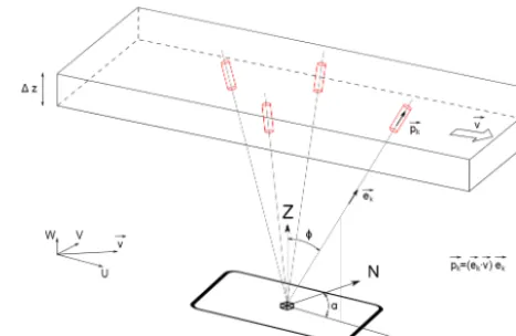
For a given azimuthαand zenith angleφ, the beam direction can be described by a unit vector given as
e=
sinαsinφ
cosαsinφ
cosφ
∈R 3.
The goal is to retrieve an unknown wind vectorv∈R3from projections ofv on a set of different beam vectors{ek}Nk=1.
Figure 1.Schematics of sampling forN=4.
This set of beam vectors defines the spatial sampling. The assumption is that within the sampling volume and sampling time the wind vector to be determined v∈R3 is constant, i.e. within the sampling volume we assume a constant wind. This assumption appears to be overly restrictive, but the goal is not to determine the instantaneous wind vector in an ar-bitrary turbulent wind field, but rather the mean (horizontal) wind vector over an averaging time ofO(10–30 min). For the average wind field, horizontal homogeneity has to be as-sumed over the area spanned by the beam directions, which is for Doppler profilers typicallyO(0.1–10 km), and stationar-ity has to be assumed over the averaging time. In the vertical, the wind field is assumed to be piecewise constant over lay-ers with a thickness of the order of the radial resolution of the Doppler profiler, namelyO(10–100 m).
The sampling process can be described through the appli-cation of projection matrices. Geometrically the projection of a vectorvonto a vectorecan be described by the 3×3 matrix
P =eeT, which easily follows since the projection ofvonto
ecan be expressed ashe,vie=ehe,vi =eeTv=Pv, where h·,·i denotes the inner product; i.e. for two given vectors
a,b∈R3 we have ha,bi =P3
i=1=ai·bi=aTb. By
con-struction, the projectionP is a rank one matrix, and, more-over,Pis idempotent and symmetric; i.e.P P=P andPT =
P. Assume now that the spatial sampling consists ofNbeam vectors, e1, . . .,eN, for which we can associate N
projec-tions,P1, . . ., PN. Each beam direction provides us with one
radial velocity vector, denoted bypk,k=1, . . ., N; hence for eachkwe can write a 3×3 linear system,pk=Pkv. Note
that the magnitude ofpk is equal to the (radial) component of the wind field in the beam direction. Combining allN lin-ear systems into one single system results in
p1 .. . pN
| {z }
p
=
P1
.. . PN
| {z }
P
wherep∈R3N andP ∈R3N,3. As each Pk is of rank one
and as we are usually faced with noisy measurements, di-rectly solving Eq. (1) is impossible. A stable retrieval of v
can be achieved through a minimization ofkp−Pvk2with respect tov. The optimalv is given through the solution of the normal equation:
(PTP )v=PTp. (2)
A unique solution requires invertibility of PTP in Eq. (2), which can be achieved if the rank of PTP equals three. Hence, at least three linearly independent beam directions are (obviously) required to obtain a unique solution. To obtain feasible numerical approximations of v, one has to ensure numerical stability of the inversion process especially in the case of noisy data; i.e. we have to ensure reasonable approx-imation quality also for the case p=p+ withkk ≤δ. As we have to solve the normal equation, we first express the symmetric map PTP by its eigensystem,PTP =U DUT, whereU is the orthogonal matrix of eigenvectors of PTP
andD=diag(λ1, λ2, λ3)is the diagonal matrix of eigenval-ues ofPTP. Then, it follows that
v=(PTP )−1PTp=U D−1UTPTp. (3)
Withv=(PTP )−1PTp, we obtain
kv−vk ≤ k(PTP )−1PT(p−p)k ≤ kU D−1UTPTk (4) kk ≤ kUkkD−1kkUTkkPTkδ≤ δ
λmin
,
whereλmin denotes the smallest eigenvalue. Therefore, the recovery error can be minimized by maximizing the small-est eigenvalue of PTP. This can be achieved by a proper choice of the corresponding beam vectorse1, . . .,eN. Hence,
the main question to answer is how to set up the beam vectors determining the spatial sampling.
2.2 Frame-based recast of the sampling design
In order to answer this question, we consider the set of beam vectors as a frame. Without mathematical rigour, a frame can be seen as a collection of vectors that span the full vector space and which are not necessarily linearly independent. Such a system of vectors is called overcomplete or redun-dant and allows given vectors to be represented in differ-ent ways (non-uniqueness). The redundancy has useful error-suppressing effects. Using this approach, the goal is to find a simple description of reconstruction stability and reconstruc-tion error dependent on the sampling design.
A set of vectors{ek}Nk=1forms a frame forR3if there exist constants 0< A≤B <∞, the so-called frame bounds, such
that for allv∈R3
Akvk2≤
N
X
k=1
|hv,eki|2≤Bkvk2 or, equivalently, (5)
hAv,vi ≤ hSv,vi ≤ hBv,vi,
whereS is the frame operator introduced below. This frame condition ensures first that all radial components have finite energy and second that the set of beam directions is com-plete; i.e. there exists no (wind) vector inR3that is
orthogo-nal to all beam directions.
Let us first reformulate the reconstruction problem. Let
e1, . . .,eN∈R3 denote the individual unit vectors of beam
directions, and consider the so-called pre-frame operatorT :
RN→R3, Tc=PNk=1ckek, with adjoint T∗:R3→RN,
given byT∗= {h·,eki}Nk=1. Then the frame operator defined asS=T T∗:R3→R3is given by
S=
N
X
k=1
h·,ekiek , (6)
which is self-adjoint and symmetric. The frame operator (Eq. 6) relates to the above-mentioned projections as follows:
S=T T∗=P1+. . .+PN=P1P1+. . .+PNPN (7)
=P1TP1+. . .+PNTPN=PTP ,
and thus the invertibility ofS is ensured by selecting three linearly independent projections (as already mentioned). In what follows we aim to elaborate how the number of beam directions might change the frame bounds ofS, which coin-cide with the smallest and largest eigenvalues ofPTP; i.e. for the bounds in Eq. (5) we haveA=λminandB=λmax.
In order to provide an explicit computation of the solution and therewith an explicit stability analysis, we recast the opti-mization problem by means of the pre-frame operatorT; i.e. we aim to find an equivalent formulation forkp−Pvk2
R3N. First, we haveT∗=(e1, . . .,eN)T :R3→RN, and bypk=
ekVk=ek(ek)Tv=Pkvthe normal equation reads as
Sv=T T∗v=TV , (8)
whereV∈RN is comprised of the radial wind components for the given beam configuration; see e.g. Päschke et al. (2015). This holds true due to
PTPv=Sv=
N
X
k=1
hv,ekiek (9)
= e1 . . . eN
(e1)T
.. . (eN)T
v
The equivalence of the optimization problems is immediate,
kp−Pvk2 R3N=
N
X
k=1
kekVk−ek(ek)Tvk2R3 (10)
=
N
X
k=1
Vk−(ek)Tv
2
= kV−T∗vk2 RN ,
and we have a reduction of dimension by a factor of 3.
3 Explicit solution and error analysis
In practice, the linear system (Eq. 3) can be solved numer-ically through the singular value decomposition (see e.g. Päschke et al., 2015), to minimize errors from finite computa-tional accuracy. This method provides numerical solutions in the general case, and it can therefore be implemented in op-erational Doppler systems. Nevertheless, an explicit solution of Eq. (3) would provide more insight into error propagation and thus allow a further investigation of optimal sampling conditions. Such an explicit solution can indeed be given for a VAD-like sampling scenario. In the following section it is shown that all the involved quantities and error bounds can be explicitly calculated. As these error bounds depend di-rectly on the sensing parameters, the sampling design can be optimized towards a minimal error in the retrieval.
3.1 Equispaced circular VAD-like sampling
With pre-assigned equispaced azimuth anglesαk=2π k/N,
k=0, . . ., N−1 and constant zenith angleφwe have
T∗=
sinα0sinφ cosα0sinφ cosφ
.. .
sinαN−1sinφ cosαN−1sinφ cosφ
, (11)
V =
V0
.. . VN−1
,v=
u v w
.
The minimization of kV−T∗vk2 results in Sv=TV or, equivalently, in PTPv=PTp. Hence, in order to provide an explicit expression for the solution of this linear system, we have to derivePTP, which is given by
PTP= (12)
PN−1
k=0sin2αksin2φ PNk=0−1sinαkcosαksin2φ PkN=0−1sinαksinφcosφ PN−1
k=0sinαkcosαksin2φ PNk=0−1cos2αksin2φ PkN=0−1cosαksinφcosφ PN−1
k=0sinαksinφcosφ PNk=0−1cosαksinφcosφ PNk=0−1cos2φ
.
The key for evaluating this matrix is interpreting each of the entries as finite geometric series. Therefore, with the help of the following summations,
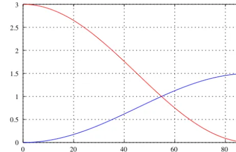
Figure 2.Plot of N2sin2φ(blue) andNcos2φ(red) forN=3.
N−1 X
k=0
sin2αk= N−1
X
k=0
eiαk−e−iαk
2i
2 =N
2
N−1 X
k=0
cos2αk= N−1
X
k=0
eiαk+e−iαk
2
2 =N
2
N−1 X
k=0
sinαk= N−1
X
k=0
eiαk−e−iαk
2i =0
N−1 X
k=0
cosαk= N−1
X
k=0
eiαk+e−iαk
2 =0
N−1 X
k=0
sinαkcosαk= N−1
X
k=0
eiαk−e−iαk
2i
eiαk+e−iαk
2
=0,
the matrixPTP simplifies to
PTP =S=
N
2sin
2φ 0 0
0 N2sin2φ 0
0 0 Ncos2φ
. (13)
This means that the frame operatorSis diagonal for eachφ
andN≥3 with frame bounds (see Fig. 2)
A=λmin=min N
2sin
2φ, Ncos2φ
, (14)
B=λmax=max N
2sin
2φ, Ncos2φ.
In the case ofA=B, i.e. sin2φ=2cos2φ, the frame is called tight. The corresponding φ then satisfies sin2φ=2/3 and hence φtight=arcsin
√
2/3≈54.7356. The wind retrieval vector is now easily computed as
v=S−1PTp=S−1TV, (15)
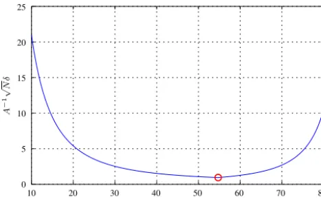
Figure 3.Frame bounds dependent on the angleφ (forN=10). The red circle indicates the minimum forφtight=arcsin
√
2/3.
S−1=
2
Nsin
−2φ 0 0
0 N2sin−2φ 0
0 0 N1cos−2φ
(16)
with bounds forφ < φtight:B−1=Ncos12φandA
−1= 2
Nsin2φ,
forφ > φtight:B−1= 2
Nsin2φandA
−1= 1
Ncos2φ, and forφ=
φtight:A=B=N3.
With the help of Eqs. (15) and (16), the explicit algebraic solution is obtained as
v=
2
Nsin2φ 0 0
0 2
Nsin2φ 0
0 0 1
Ncos2φ
(17)
sinα0sinφ . . . sinαN−1sinφ cosα0sinφ . . . cosαN−1sinφ
cosφ . . . cosφ
V0 .. . VN−1
.
The matrix multiplications in Eq. (17) of the inverse frame operatorS−1with the pre-frame operatorT, whose columns are comprised of the unit vectors describing the beams, yield the explicit solution for the wind vector:
v= u v w = 2
Nsinφ
PN−1
k=0 sinαkVk
2
Nsinφ
PN−1
k=0 cosαkVk
1
Ncosφ
PN−1
k=0Vk
. (18)
3.2 Estimation of the retrieval error
Since the wind retrieval for the equispaced VAD sampling case can be explicitly expressed asv=S−1TV, it is possible to investigate the propagation of measurement errors in the radial wind components to the final wind vector directly. In
what follows, the deterministic as well the stochastic error model will be discussed.
Assume, as before, the deterministic error model Vδ=
V+1V, where k1Vk ≤δ. For the reconstruction error we then obtain1v=vδ−v=S−1T (Vδ−V)=S−1T 1V, which is
1v=S−1
sinφPN−1
k=0 sinαk1Vk
sinφPN−1
k=0 cosαk1Vk
cosφPN−1
k=01Vk
. (19)
Therefore, with the help of the Cauchy–Schwarz inequality,
k1vk2≤ kS−1k2
sin2φ
N−1 X
k=0
sinαk1Vk
!2
(20)
+sin2φ
N−1 X
k=0
cosαk1Vk
!2
+cos2φ
N−1 X
k=0
1Vk
!2
≤ kS−1k2hsin2φN
2k1Vk
2+sin2φN 2k1Vk
2
+cos2φNk1Vk2i≤A−2N δ2.
Consequently, from Eq. (20) we deduce
k1vk ≤A−1
√
N δ= 2δ √
Nsin2φ for φ < φtight
3δ
√
N for φ
=φtight
δ
√
Ncos2φ for φ > φtight
. (21)
The essential observation in Eq. (21) is that an increase of the number of beams leads to a smaller reconstruction error and that the smallest error (for anyN) is achieved forφ=φtight; see Fig. 3.
Now assume that the measured radial wind components follow the simple stochastic model, Vδ=V+1V, with
1V∼N(β,6), whereN(β,6)is theN-dimensional nor-mal distribution with expectation vectorβand variance ma-trix6. If we assume that the components ofβare constant,
βi=β for i=0, . . ., N−1, and 6=diag(σ2, . . ., σ2). By
computing the expectation of the bias,E(1v), one obtains
E(1v)=E(S−1T 1V)=S−1T E(1V)=S−1Tβ (22)
=S−1
sinφPN−1
k=0 sinαkβ
sinφPN−1
k=0 cosαkβ
cosφPN−1
k=0β = β cosφ 0 0 1 .
To compute the mean square error (MSE), standard argu-ments lead to
E(1v1vT)=S−1T E(1V1VT)TTS−1
=S−1T (6+ββT)TTS−1
=Var(1v)+(E1v)(E1v)T
| {z }
bias2
,
which is clear due to 6j k=E(1Vj−β)(1Vk−β)=
E1Vj1Vk−β2, which is obvious as by independency it
holds forj 6=kthatE1Vj1Vk=E1Vj·E1Vk=β2, and
therefore
E1Vj1Vk=
σ2+β2, j =k β2, j6=k.
In the stochastic regime, the deterministic error estimate can be reproduced. Indeed, it can be observed that
Ek1vk2≤ kS−1k2 sin2φX
j k
(sinαjsinαk+cosαjcosαk)
E1Vj1Vk+cos2φ
X
j k
E1Vj1Vk
!
= kS−1k2N (σ2+β2)+ kS−1k2β2
sin2φ NX k
cos(2π k/N )−N !
+N (N−1)cos2φ !
= kS−1k2N (σ2+β2)+ kS−1k2β2N (Ncos2φ−1)
=A−2N σ2+A−2N2β2cos2φ.
This estimate verifies the deterministic recovery error, and for growingN this error component can also be made arbi-trarily small. The second summand, however, cannot be com-pensated as it is independent ofN.
The MSE can be explicitly calculated as follows:
Ek1vk2=E(1u)2+(1v)2+(1w)2 (23)
= 4
N2sin2φ X
j k
(sinαjsinαk+cosαjcosαk)
E1Vj1Vk+
1
N2cos2φ X
j k
E1Vj1Vk
!
=
4
N2sin2φN σ
2+ 1
N2cos2φ(N σ
2+N2β2)
=σ 2
N
4 sin2φ
+ 1 cos2φ
+ β
2
cos2φ.
Forβ=0 and fixedN, the choiceφ=φtightyields the small-est value for the MSE. The caseβ6=0 changes the situation. Let
Ek1vk2=σ 2
N
4sin−2φ+c·cos−2φ
| {z }
=:F (φ)
,
wherec=1+Nβ2
σ2. For extremal values,F
0(φ)=0 must be
evaluated, which is equivalent to evaluating
(4−c)sin4φ−8sin2φ+4=0.
We obtain sin2φ=(4−2√c)/(4−c)=2/(2+√c), which is equivalent to tan2φ=2/√c, and consequently
φ=arctan s
2 √
c. (24)
Equation (24) provides us for each givenN,βandσ with an optimal (MSE-minimizing) zenith distance angleφ.
Finally, from the computation ofEk1vk2 in Eq. (23) it follows that
E
(1u)2 (1v)2 (1w)2
=
2σ2
Nsin2φ
2σ2
Nsin2φ σ2
Ncos2φ
+
0 0
β2
cos2φ
, (25)
supporting and explaining results obtained by Cheong et al. (2008), who have experimentally shown that the MSE or likewise the RMSE of the wind retrieval is significantly re-duced by increasing the number of off-vertical beams in the Doppler beam-swinging technique in the presence of wind field inhomogeneities. Note, however, that for the vertical wind component only the random error can be reduced by an increase ofN.
4 Conclusions
In this note, the mathematical concept of frames is applied to the analysis of the spatial (beam configuration) sampling setup for Doppler profilers for the case of a horizontally homogeneous and stationary wind field. It could be shown that it is possible to derive a compact explicit least-squares wind retrieval solution for a typical symmetric VAD scan-ning scheme. Such an explicit formula had hitherto not been published yet. Besides its simplicity, it allows for a straight-forward stability analysis in the practically relevant case of noisy data. The explicit solution exhibits the known fact that the VAD-based estimate for the horizontal wind components is unbiased even if the radial wind components have a con-stant (direction-independent) bias. Furthermore it was shown that the MSE retrieval error is∝1/N up to a constant offset due to the bias, which means that a larger number of off-zenith beam directions is beneficial to reduce the variance of the wind vector components. The total retrieval error is de-pendent upon the zenith angleφ. For the most relevant case
β=0 it is minimal if the beam vectors form a tight frame. The optimal beam zenith angle for this case was calculated as
systems. However, it is important to appreciate that for the practically relevant case of an estimate of only the horizon-tal components of the mean wind (since the mean vertical wind component will mainly be close to zero, except for spe-cial meteorological conditions) no such optimum can be de-rived from purely geometrical arguments. Another reason to deviate from this optimal elevation angle is due to the re-quirement to keep the sampled volume small, in an attempt to minimize deviations from a constant wind field. Technical constraints like the usable Nyquist velocity range and lim-ited scanning capabilities of phased array radar antennas are further reasons why the theoretically optimal elevation is not used in practice.
Data availability. No data sets were used in this article.
Competing interests. The authors declare that they have no conflict of interest.
Acknowledgements. We appreciate the efforts of the editor and the two anonymous reviewers, whose comments helped to improve this paper.
Edited by: Laura Bianco
Reviewed by: two anonymous referees
References
Browning, K. and Wexler, R.: The Determination of Kinematic Properties of a Wind Field Using Doppler Radar, J. Appl. Me-teorol., 7, 105–113, 1968.
Caya, D. and Zawadzki, I.: VAD Analysis of Nonlinear Wind Fields, J. Atmos. Ocean. Tech., 9, 575–587, 1992.
Cheong, B. L., Yu, T.-Y., Palmer, R. D., Yang, K.-F., Hoffman, M. W., Frasier, S. J., and Lopez-Dekker, F. J.: Effects of Wind Field Inhomogeneities on Doppler Beam Swinging Revealed by an Imaging Radar, J. Atmos. Ocean. Tech., 25, 1414–1422, 2008. Christensen, O.: Frames and Bases. An Introductory Course, Ap-plied and Numerical Harmonic Analysis, Birkhäuser, Boston, 2008.
Cifelli, R., Rutledge, S. A., Boccippio, D. J., and Matejka, T.: Hor-izontal Divergence and Vertical velocity Retrieval from Doppler Radar and Wind Profiler Observations, J. Atmos. Ocean. Tech., 13, 948–966, 1996.
Davidson, P. A.: Turbulence, Oxford Univ. Press., New York, 2004. Dutton, J. A.: The Ceaseless Wind, Dover Publications, New York,
1986.
Fuertes, F. C., Iungo, G. V., and Porté-Agel, F.: 3D Turbulence Mea-surements Using Three Synchronous Wind Lidars: Validation against Sonic Anemometry, J. Atmos. Ocean. Tech., 31, 1549– 1556, 2014.
Holleman, I.: Quality Control and Verification of Weather Radar Wind Profiles, J. Atmos. Ocean. Tech., 22, 1541–1550, 2005. Koscielny, A. J., Doviak, R. J., and Zrnic, D. S.: An Evaluation
of the Accuracy of Some Radar Wind Profiling Techniques, J. Atmos. Ocean. Tech., 1, 309–320, 1984.
Larsén, X. G., Larsen, S. E., and Petersen, E. L.: Full-Scale Spec-trum of Boundary-Layer Winds, Bound.-Lay. Meteorol., 159, 349–371, 2016.
Maurer, V., Kalthoff, N., Wieser, A., Kohler, M., Mauder, M., and Gantner, L.: Observed spatiotemporal variability of boundary-layer turbulence over flat, heterogeneous terrain, At-mos. Chem. Phys., 16, 1377–1400, https://doi.org/10.5194/acp-16-1377-2016, 2016.
Newman, J. F., Klein, P. M., Wharton, S., Sathe, A., Bonin, T. A., Chilson, P. B., and Muschinski, A.: Evaluation of three lidar scanning strategies for turbulence measurements, Atmos. Meas. Tech., 9, 1993–2013, https://doi.org/10.5194/amt-9-1993-2016, 2016.
Päschke, E., Leinweber, R., and Lehmann, V.: An assessment of the performance of a 1.5 µm Doppler lidar for operational vertical wind profiling based on a 1-year trial, Atmos. Meas. Tech., 8, 2251–2266, https://doi.org/10.5194/amt-8-2251-2015, 2015. Salby, M. L.: Fundamentals of Atmospheric Physics, International
Geophysics Series, Academic Press, 1996.
Sathe, A. and Mann, J.: A review of turbulence measurements using ground-based wind lidars, Atmos. Meas. Tech., 6, 3147–3167, https://doi.org/10.5194/amt-6-3147-2013, 2013.
Sathe, A., Mann, J., Vasiljevic, N., and Lea, G.: A six-beam method to measure turbulence statistics using ground-based wind lidars, Atmos. Meas. Tech., 8, 729–740, https://doi.org/10.5194/amt-8-729-2015, 2015.
Shenghui, Z., Ming, W., Lijun, W., Chang, Z., and Mingxu, Z.: Sen-sitivity Analysis of the VVP Wind Retrieval Method for Single-Doppler Weather Radars, J. Atmos. Ocean. Tech., 31, 1289– 1300, 2014.
Stephens, G. L.: Remote Sensing of the Lower Atmosphere, Oxford University Press, New York, 1994.
Stull, R. B.: An Introduction to Boundary Layer Meteorology, Kluwer Academic Publisher, 1988.
Vallis, G. K.: Atmospheric and Ocean Fluid Dynamics, Cambridge University Press, 2006.
Waldteufel, P. and Corbin, H.: On the Analysis of Single-Doppler Radar Data, J. Appl. Meteorol., 18, 532–542, 1979.
Warner, T. T.: Numerical Weather and Climate Prediction, Cam-bridge University Press, New York, 2011.