Adaptive Filtering using Steepest Descent and LMS Algorithm

Adaptive Filtering using Steepest Descent and

LMS Algorithm

Akash Sawant Pratik Nawani

Department of Electronics & Telecommunication Engineering Department of Electronics & Telecommunication Engineering Mukesh Patel School of Technology Management and

Engineering, NMIMS University, Mumbai, India

Mukesh Patel School of Technology Management and Engineering, NMIMS University, Mumbai, India

Shivakumar

Department of Electronics & Telecommunication Engineering

Mukesh Patel School of Technology Management and Engineering, NMIMS University, Mumbai, India

Abstract

In many practical scenarios, it is observed that we are required to filter a signal whose exact frequency response is not known. A solution to such problem is an adaptive filter. It can automatically acclimatize for changing system requirements and can be modelled to perform specific filtering and decision-making tasks. This paper primarily focusses on the implementation of the two most widely used algorithms for noise cancelling which form the crux of adaptive filtering. The empirical explanation of steepest descent method is elucidated along with its simulation in MATLAB by taking a noise added signal and applying the ingenuity of this algorithm to get the desired noise-free response. Furthermore, this paper also sheds light on a more sophisticated algorithm which is based on the underlying criteria of minimum mean square error called as the Least Mean Square (LMS). Additionally, there are various applications of adaptive filtering including system identification which is briefly explained to emphasize the instances where it can be used.

Keywords: Steepest Descent, LMS, Mean Square Error, Tap Weights, Stochastic Gradient Algorithm

________________________________________________________________________________________________________

I.

I

All physical systems produce noise while operating in a dynamic environment and subsequently corrupt the information. The complexity of the signal makes it difficult to comprehend for the human ear or other system through which this acts as the input. This leads to the advent of an algorithm which is capable of separating this noise from the desired response called as the adaptive filtering algorithm. It can be deployed in fast-changing and unknown environments to reduce the noise level as much as it can. An adaptive filter is the one that solves this complication by employing such algorithms. It is a computational device that repeatedly models the relationship between the input and output signals of the filter. It is a self-designing and time-varying system that uses a recursive algorithm continuously to adjust its tap weights for operation in an unknown environment. This makes the adaptive filter more robust than a conventional digital filter. A conventional digital filter has only one input signal u(n) and one output signal y(n), whereas an adaptive filter requires an additional input signal d(n); called the desired response and so it also returns an additional output signal e(n) which is the error signal. The filter coefficients of an adaptive filter is updated over time and have a self-learning ability that is absent in conventional digital filters. Self-adjustments of the filter coefficients are done by using an algorithm that changes the filter parameters over time so as to adapt to the changing signal characteristics and thus reducing the error signal e(n). But, implementing this procedure exactly requires knowledge of the input signal statistics, which are usually unknown for real-world problems. Instead, an approximate version of the gradient descent procedure can be applied to adjust the adaptive filter coefficients using only the measured signals. Such algorithms are collectively known as stochastic gradient algorithms which are explained further along with the MATLAB simulation of steepest descent algorithm.

II.

S

The modus operandi of the method pivots on the point that the slope at any point on the surface provides the best direction to move in. It is a feedback approach to finding the minimum of the error performance surface. The steepest descent direction gives the greatest change in elevation of the surface of the cost function for a given step laterally. The steepest descent procedure uses the knowledge of this direction to move to a lower point on the surface and find the bottom of the surface in an iterative manner.

III.

M

d(n)= WT(n)X(n)

where X(n) = [x(n) x(n−1) ··· x(n−L + 1)]T is a vector of input signal samples and W(n) = [w0(n) w2(n) ··· wL−1(n)]T is a vector containing the coefficients or the weights of the FIR filter at time n.

Now, the coefficient vector W(n) needs to be found out that optimally replicates the input-output relationship of the unknown system such that the cost function of the estimation error given by

e(n) = d(n)- d(n) is the smallest among all possible choices of the coefficient vector.

An apt cost function is to be defined to formulate the steepest descent algorithm mathematically. The mean-square-error cost function is given by

J(n) = E{((e(n))2} =E{(d(n)−WT(n)X(n))2} Where J(n) is the non- negative function of the weight vector.

Step 1: in order to implement the steepest descent algorithm, the partial derivatives of the cost function are evaluated with respect to the coefficient values. Since derivatives and expectations are both linear operations, we can change the order in which the two operations are performed on the squared estimation error.

{ ( )}

( ) = E(2e(n)

( ) ( )) = -2E{e(n)X(n)}

Step 2: Finding the difference in the coefficient vector of two consecutive time spaced weights which forms the basis for the algorithm.

W (n + 1) = W (n) + µE{e(n)X(n)} Where µ is step size of the algorithm and

∆W= W (n + 1) – W (n) Step 3: Determining the expectation from the above equation

E{e(n)X(n)} = E{X(n)(d(n)−d(n))} = Pdx(n)−Rxx(n)W(n)

Where Rxx(n) is autocorrelation matrix of input vector and the cross correlation matrix vector of the desired response signal and the input vector at time n is indicated by Pdx(n) . The optimal coefficient vector is found out when the estimation error or ∆W is zero.

W opt (n) = Rxx-1(n) PdX (n)

The aim is to iteratively descend to the bottom of the cost function surface, so that W(n) approaches Wopt(n) i.e. the coefficient vector is updated repetitively using a strategy analogous to that of the ball rolling in a bowl.

IV.

S

From the figure, the following facts become evident:

1) The slope of the function is zero at the optimum value associated with the minimum of the cost function. 2) There is only one global minimum of the bowl- shaped curve and no local minima.

3) The slope of the cost function is always positive at points located to the right of the optimum parameter value.

4) For any given point, the larger the distance from this point to the optimum value, the larger is the magnitude of the slope of the cost function.

Fig. 1: Mean Square Error Cost Function For A Single Coefficient Linear Filter

will make smaller adjustments when the value is close to the optimum value. This approach is the essence of the steepest descent algorithm. The filter coefficients are successively updated in the downward direction, until the minimum point, at which the gradient is zero, is reached.

V.

M

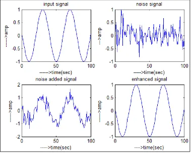
The steepest descent method is implemented in MATLAB with a signal added with noise which is filtered by execution of the algorithm.

Fig. 2: MATLAB Implementation of Steepest Descent Method

The input signal being a sinusoidal wave corrupted with a deliberately added White Gaussian noise is taken as input upon which the code is implemented which adjusts the tap weight and minimizes the error signal e(n). The noise added signal is the n filtered off iteratively giving the enhanced signal as the output.

VI.

L

The least-mean-square (LMS) algorithm is part of the group of stochastic gradient algorithms. The update from steepest descent is straightforward while the dynamic estimates may have large variance; the algorithm is recursive and effectively averages the estimate values. The simplicity and good performance of the LMS algorithm makes it the benchmark against which other optimization algorithms are judged. This algorithm is prevalent amongst various adaptive algorithms because of its robustness. It is based on the MMSE (Minimum Mean square Error) criterion. The LMS algorithm is based on the concept of steepest-descent that updates the weight vector as follows:

w(n + 1) = w(n) + μ(X(n)e(n))

Where μ is the step size (or convergence factor) that determines the stability and the convergence rate of the algorithm

The comprehensibility of the algorithm lies in the fact that it doesn’t require the gradient to be known; implying that it is estimated at each iteration; unlike in the steepest descent approach. The expectation operator is ignored from the gradient estimate,

{ ( )}

( ) is replaced by ( ) ( )

Now, in order to update the coefficients by using instantaneous gradient approximation in the LMS Algorithm; we get the following equation for error e(n);

e(n) = d(n) - WT(n)X(n)

The LMS Algorithm consists of two basic processes:

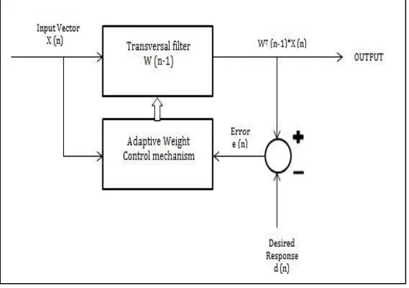
Filtering Process: A.

This step entails calculating the output of FIR transversal filter by convolving input and tap weights. A transversal filter which is used to compute the filtered output and the filter error for a given input and desired signal. Subsequently, the estimated error is found out by comparing the output signal to the desired response.

Fig. 3: Lms Filtering Process

Adaptation Process: B.

This is a simultaneous operation during implementation as it adjusts tap weights based on the estimated error. This adjustment is done via a control mechanism which contains vector X (n) as its input. It can be represented by the formula as:

W (n+1) = W (n)-µ { ( )} ( ) It is approximated to

W (n+1) = W (n) + 2µe (n) X (n) Thus, the tap weight W (n+1) is altered based on the error e (n) and the step size µ.

Fig. 4: LMS Adaptation Process

VII.

S

The minimum mean square criterion of LMS algorithm is satisfied if and only if the step-size parameter satisfy

Here max is the largest eigenvalue of the correlation matrix R of the input data

However, in practicality the eigenvalues of R are not known, so the sum of the eigenvalues (or the trace of R) is used to replace λmax. Therefore, the step size is in the range of 0 < μ < 2/trace(R).

Since trace(R) = MPu which is the average power of the input signal X (n), a commonly used step size bound is obtained as Thus, a more pragmatic test for stability is

The larger values for step size have a trade-off. It increases the adaptation rate but, on the other hand, this leads to increase in the residual mean-squared error.

VIII.

A

Adaptive filters can be configured in a large variety of ways for a large number of applications and it is perhaps the most important driving forces behind the developments in dynamic filtering. Adaptive filters are used in several applications because of their ability to function in unfamiliar and varying environments and one of which is system identification. The primary goal of adaptive system identification is to approximate or determine a discrete estimation of the transfer function of an unknown system. The adaptive filter helps in providing a linear representation that is the best approximation of the unknown system.

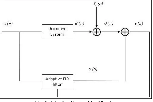
Fig. 5: Adaptive System Identification

The adaptive system identification configuration is shown in the figure above, where we can see that an adaptive FIR filter is kept in parallel with an unknown digital or analog system which we want to identify. The input signal x (n) of the unknown signal is commensurate with the input signal x (n) of the adaptive FIR filter, while the ƞ (n) represents the disturbance or the noise signal occurring within the unknown system. Let d (n) represent the output of the unknown system with x (n) as input. Therefore the desired signal in this model is given by

d (n) = đ (n) + ƞ (n)

The purpose of the adaptive filter is to accurately represent the signal đ (n) as its output. If the adaptive filter is able to make y (n) = đ (n), then the adaptive filter has successfully and accurately identified the part of the unknown system that is driven by x (n). This can be accomplished by minimizing the error signal e (n), which is the difference between the output of the unknown system and the adaptive filter output y (n). The adaptive system identification is widely applied in plant identification, channel identification, echo cancellation for long distance transmission, adaptive noise cancellation, acoustic echo cancellation.

IX.

C

We have discussed the implementation of the most widely used algorithms in adaptive filtering pertaining to the noise cancellation along with its simulation in MATLAB. This paper provides a reference for understanding the concept of steepest descent and LMS methods. But, the concept of adaptive filtering is not only limited to the purview of noise cancellation and system identification as it is elicited in the paper. Also, it finds its uses in inverse modelling, linear prediction and spectral analysis of speech signals. The recent advancements under this domain have really shaped the way signal processing is done.

R

[1] Kong-Aik Lee, W.-S. G. (2009). Subband Adaptive Filtering: Theory and Implementation. John Wiley & Sons, Ltd.

[2] O.Macchi. (1995). Adaptive Processing: The Least Mean Squares Approach with Applications in Transmission. Wiley.

[3] S.Haykin. (2002). Adaptive Filter Theory. Prentice-Hall.