Designs of Second-Order Associated Memory
Networks with Threshold Logics:
Winner-Take-All and Selective Voting
Toshiro Kubota
Department of Mathematical Sciences, Susquehanna University, Selinsgrove PA, USA Email: [email protected]
Abstract— The capacity of an order-d associative memory model is O(Nd/logN)where N is the memory size in bit. In contrast, the capacity of the Hopfield network is limited
to O(N/logN). Among higher order associative memory
models (d > 1), the second order memory (d = 2) has attractive properties: a relatively small implementation cost of O(N2), a small number of spurious states, and the presence of a diagonalization form. Due to these properties, it is of both practical and scientific interests to investigate efficient computational mechanisms of such network.
One disadvantage of higher order associative memory is that it cannot be implemented with simple threshold neurons or McCulloch-Pitts neurons, thus a direct implementation of its computational mechanism on a biological substrate is questionable and its silicon implementation is expensive. In this paper, we propose two approximation models of a second order associative memory using threshold logics. Both are two-layered and employ eigenvalue decomposition of the correlation tensor. The first model uses a winner-take-all mechanism and the second uses a weighted voting by those with significant responses. Architectural-level designs of these memory models are presented. Extensive numer-ical simulations demonstrate effectiveness of the proposed models in retrieving contents with noisy probe vectors.
Index Terms— neural networks, memory capacity, error correction, architectural level design
I. INTRODUCTION
Associative memory has been consistently an active research area since the works of Kohonen [1], Cohen and Grossberg [2], and Hopfield [3]. Most efforts have been directed to increase the memory capacity, improve the error correction capability, reduce the number of spurious memories, and improve biological feasibility [4] [5] [6] [7]. Advances in this field may reveal important aspects of brain and perception of animals including humans.
Two popular extensions to a Hopfield type network for improving the memory capacity are introduction of self-feedback and relaxation of the synaptic weights to asymmetric ones. In [5], Gorodnichy demonstrated that the size of the attraction basin could be increased with a proper amount of self-feedback in a network trained with the pseudo-inverse learning. Similarly in [8], it was shown
This paper is based on “Second Order Associative Memory Models with Threshold Logics - Eigen Mode Selections,” by T. Kubota, which appeared in the Proceedings of the IEEE International Conference on Systems, Man, and Cybernetics (SMC), Montreal, Canada, October 2007. c2007 IEEE.
that a small amount of self-feedback could reduce the number of spurious states in Hopefield networks. More-over, in [7], empirical studies of Hopfield networks with asymmetric additive random weights were conducted. The study showed that the asymmetric weights reduced the number of spurious states while no significant change to the size of attraction basins.
A number of learning algorithms have been suggested to replace the traditional Hebbian and Pseudo inverse learning rules. In [9], the authors proposed a Perceptron type learning algorithm with a goal of maximizing a stability measure of the memory. In [8], additional training vectors were introduced systematically so as to increase the size of the attraction basin with the learning algorithm of [9].
A more drastic departure from the traditional first-order correlation memory has been shown to improve the retrieval performance of the memory. Memory models with higher order correlation have been explored and shown to increase the capacity from O(N/logN) of the Hopfield model to O(Nd/logN) where N is the number of neurons in the model and d is the order of the correlation [10] [11] [12]. However, biological feasibility of such systems is questionable as evaluation of a polynomial of order d is required for each memory cell or neuron.
In this paper, we discuss how to arrange the compu-tational mechanism of a higher-order associative memory so that it can be approximated with a collection of simple neuron models. Considering biological feasibility and cost-effective silicon implementation in mind, we impose the following design requirements.
1) Each neuron can compute a sum of binary inputs weighted by real numbers.
2) Each neuron can perform a generalized threshold operation to the weighted sum to produce a binary output. The operation is defined as
χ(z) =
⎧ ⎨ ⎩
∆+ z > θ ∆− z <−θ
∆0 otherwise
(1)
where∆• are either 1, -1 or ±the current neuron state, andθ is a threshold value.
The model is a slightly generalized version of the McCulloch-Pitts neuron. The threshold operation (1) can accommodate both the original Hopfield model and high-correlation order memories of [10] [11]. To specify the threshold operation, we use symbols {+,−,◦,↑} to de-scribe specific ∆•. The symbols indicate 1, -1, x and −x, respectively, with x being the state of the neuron. Furthermore, we compactly writeχ(z;θ,∆−,∆+,∆0)to
fully describe the threshold operation.
When these computational requirements are met, the system can be constructed with a set of simple processing elements that are often considered biologically feasible [13] [14] and amiable to implementation on silicon. Since each input is bipolar (i.e. the value is ±1), the weighted sum can be implemented with adders. Thus, no multipliers are required in the design. Furthermore, the communication or wiring cost is small and scalable as data transmitted between processing elements are strictly binary. The main objective of this work is in two-fold: to present approximation models of a second-order associa-tive memory and to design architectural level circuits for the approximation models.
In this paper, we consider the following scenario. The memory consists of N memory cells. During a storage phase, the memory is presented withK randomly chosen bipolar vectors ofNdimensions (i.e. each element is±1). We call them fundamental vectors. We consider that the set of fundamental vectors is given prior to a retrieval phase and remains unchanged. During the retrieval phase, the memory is initially set to a bipolar vector of length
N, which we callprobe vector, and the memory performs internal processing and settles to another bipolar vector of length N, which is the memory content retrieved by the probe vector. We only consider auto-association memory, therefore the retrieval is considered correct if the retrieved vector is one of fundamental vectors whose Hamming distance is the smallest to the probe vector.
We use the following notations. Matrices and tensors are written in upper bold letters (C, for example). Vectors are written in lower bold letters (v). Scalars are written in non-bold italic letters (xandN). Sub-scripts are used to index elements of a countable set. For example, funda-mental vectors are addresses asu1,u2, ..., anduK. They are also used to index components in vectors, matrices and tensors. A set index precedes a component index. Therefore, jth component of kth fundamental vector is addressed as ukj. Super-scripts are used to specify
particular memory cell. We use x for the state of the memory. Therefore, xi denotes the bipolar state of the
ith memory cell. We use(x,y)to denote a dot product of two vectors,xandy. Memory models run iteratively and we call each iterationepoch. To avoid ambiguity, we may attach the epoch number to the memory state and other associated variables. In the case, a number enclosed in[ ] indicates the index of the epoch. For example,xk[t]is the state ofkth memory attth epoch. Whenx[t] =x[t+ 1], the memory is said to bestable, and otherwise, it is said to beunstable.
The memory carry various signals internally, which can be either bitor multi-bit. A bit signal can be transmitted by a single-bit wire. A multi-bit signal requires a multi-bit bus to be transmitted. A bit number can be either binary or bipolar where the former carries 0 or 1 and the latter carries 1 or -1. When a bit signal is transmitted via a single wire, we need to keep in mind the semantic of the signal: binary or bipolar. The distinction between the two becomes important in designing digital circuits of the memory in Section V.
In our experiments (Section IV), we impose random noise to a probe vector. The noise level is indicated by
Q ∈ [0,1.0]. To add noise, we select QN bits in the probe vector randomly and flip their states. Finally, we call a correlation memory of orderd,d-order memory. In particular, we call 2-order and 3-order memories second order memory andthird order memory, respectively.
The paper is organized as follows. Section 2 provides background materials and brief accounts of other relevant associative memory models. Section 3 describes proposed memory models. Section 4 provides results of numerical experiments. Section 5 provides designs of the proposed memory models and compare them against those of relevant models. Finally, Section 6 provides summary and remarks. An earlier and shorter version of this paper appeared in [15].
II. BACKGROUNDS
A. Correlation Memory Models
The original Hopfield network is a fully connected re-current one and each neuron stores one bit of information. In this sense, neurons and memory cells are equivalent. It obeys the following update rule.
zi[t] = (wi,x[t]), (2)
xi[t+ 1] =χ(zi[t]; 0,+,−,+). (3)
We call zi the action potential of an ith neuron. The synaptic weights, wi, are computed with Hebbian rule without any self-feedbacks. Thus,
wij= K
k=1
ukiukj (4)
for i=j andwii= 0.
Ad-order memory uses ad-tensor,Ci, computed with an extension of the above Hebbian rule.
Ci=
K
k=1
ukiuk×uk×...×uk (5)
with a correlation tensor is
n d
. The update ofd-order
memory is
zi[t] =Ci·(x[t]×...×x[t]) (6)
xi[t+ 1] =χ(zi[t];θ,+,−,↑). (7)
where the cartesian products in (6) are repeated d−1
times and · is an inner product of d and d−1 tensors as defined in [16]. WhenCi is defined as (5), (6) can be written as
zi[t] = K
k=1
uki(uk,x[t−1])d (8)
The threshold value,θ, is set to 0 ford even andO(K)
for dodd [10]. It has been shown that the capacity of an
d-order memory is O(Nd/logN) patterns of length N
and the radius of the attraction basin approachesN/2as
N approaches ∞.
The size of a correlation tensor is O(Nd), which reflects the storage requirement imposed on each neuron. This exponential growth of the storage requirement makes a network with a large dprohibitively expensive. There-fore, in practice, we are often limited to d≤3.
Two vectors (say xandˆx) are of opposite polarities if
xi=−xˆi,∀i. It is well known that the Hopfield network cannot distinguish two vectors of opposite polarities [17]. In other words, if x is a stable/unstable state of the network, then −x is also stable/unstable. This behavior can be easily observed from the update rule of (2) and (3); Note first that the network is stable if and only ifxizi> θ, ∀i. When the sign of every component of x is flipped, then every zi will change its sign without changing its magnitude. Therefore, the condition of xizi > θ being true or false is not affected by the polarity of x. Ifx is stable, then so is −x. If x is unstable, then so is −x. Whenxis one of fundamental vector but−x is not, then we consider −x spurious as it is stable yet is not one being stored in the memory.
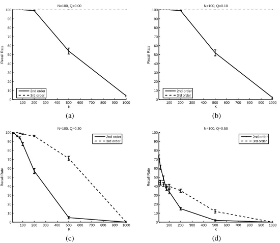
In reference to (8), we can observe that the same behavior holds for a network with an odd d but not for one with an even d. Due to this behavior, the memory recall rate of an even order network tends to be less sensitive to noise imposed on a probe vector. Figure 1 shows the memory recall rates of second order and third order memories with various Ks and Qs. The size of the network (N) is set to 100. K changes from 10 to 1000. Four levels of Q are tested: 0, 0.1, 0.3, and 0.5. The third order memory shows a larger capacity than the second order one. However the recall rate of the third order memory decreases quickly as the noise level increases. The recall rate of the second order memory is less sensitive to the noise level. The results agree with the above observation.
Due to the aforementioned practical feasibility and good error correction capability, we focus our inves-tigation to a second-order correlation network in this paper. The correlation tensor in this case is an N×N
symmetrical matrix computed by
Ci=
K
k=1
ukiukuTk. (9)
where T is a transpose operator. The update of (6) becomes
zi[t] =Ci·(x[t]×x[t]) = (Cix[t],x[t]). (10)
Since Ci is symmetrical, it can be written as
Ci=
R
k=1
λikvik
vikT (11)
where R is the rank of Ci, λk is an eigenvalue of Ci,
and vk is the corresponding ortho-normal eigenvector. This decomposition plays a critical role in developing our network models in the next section.
With (11), (10) can be expressed as
zi[t] = R
k=1
λik(vik,x[t])2. (12)
In this paper, we call each eigenvector an eigen-modeof the second order memory, the sign of λik the signof the
kth eigen-mode ofith neuron, andλik(vik,x)theresponse
of x to thekth eigen-mode. We further define
φik(x) = (vik,x) (13)
and call it the unit responseof x to thekth eigen-mode of the ith neuron.
B. Sparse Distributed Memory
Another important work on associative memory that has a similar implementation structure with second-order memory is Sparse Distributed Memory (SDM) [18].
SDM is comprised of pair-wise address and content blocks where each address holds one content. The address block contains a large collection of randomly assigned bipolar vectors whose length is N for auto-associative memory. For each address, the content block stores a vector of lengthN. The content vectors are initially set to zero. When a fundamental vector is presented to the auto-associative memory for storage, those addresses whose Hamming distances to the random vector are less than a pre-determined constant (select radius) are activated and the bipolar pattern is accumulated to the content block of the activated addresses. When a noisy probe vector is presented to the memory for retrieval, those addresses whose Hamming distances to the vector are less than the select radius are activated, and their contents are accumulated into the output buffer. A retrieved pattern is the accumulated pattern thresholded at zero. The goal of SDN is to model human cortical memories.
A critical parameter of the SDM is the select radius. Kanerva suggests in [19] that the radius be set so that the signal to noise ratio of the memory is maximized. He then go on to suggest the following formula for computing the value.
(b)
100 200 300 400 500 600 700 800 900 1000 0
10 20 30 40 50 60 70 80 90 100
K
Recall Rate
N=100, Q=0.10
2nd order 3rd order
100 200 300 400 500 600 700 800 900 1000 0
10 20 30 40 50 60 70 80 90 100
K
Recall Rate
N=100, Q=0.30
2nd order 3rd order
100 200 300 400 500 600 700 800 900 1000 0
10 20 30 40 50 60 70 80 90 100
K
Recall Rate
N=100, Q=0.50
2nd order 3rd order (a)
(c) (d)
100 200 300 400 500 600 700 800 900 1000 0
10 20 30 40 50 60 70 80 90 100
K
Recall Rate
N=100, Q=0.00
2nd order 3rd order
Figure 1. Comparing memory recall rates between second order and third order memories.
where Γn,p denotes the cumulative distribution of a bi-nomial distribution with n trials with p probability of success. In other words,
Γn,p(k) = k
j=0
n k
pj(1−p)n−j (15)
Since the binomial distribution is a discrete one, ρ is the number of successes whose cumulative probability according toΓN,0.5is closest to(2N K)−1/3.
III. MEMORYMODELS
We are interested in implementing a second order associative memory using a set of generalized threshold logics as defined in Section I. Note that the Hopfield network is implementable with the neuron models. while the second order memory is not. The latter involves multiplying two multi-bit numbers, which violates the imposed computational requirements.
For now, let’s relax the requirements and allow neurons to multiply two bit numbers and to transmit multi-bit data. Then, Equation (12) suggests a two-layered de-sign for each one bit portion of the second-order memory. The first layer consists of R neurons. Each is assigned a distinct eigen-mode of (12), and computes the unit response of its eigen-mode to the current state,x[t]. The second layer consists of a single neuron that computes the square of each incoming input, computes the sum of the first layer responses weighted by respective eigenvalues of the eigen-modes, and then takes a threshold of the result to produce a bipolar state. The result of the second layer neuron becomes the state of the bit. This is exactly the result of carrying out (12).
Figure 2 illustrates an overview of this two-layered network for a single bit memory. The first layer neurons
(Φi·) compute
yi=φik(x) =
k
vik,x). (16)
The second layer neuron (Ψi) computes
zi=
k λik
φik(x)
2=
k λik
yik
2
, (17)
xi=χ(zi; 0,+,−,↑). (18)
This model violates the requirements at three places: to take the square of a multi-bit number (yki), to multiply two multi-bit numbers (yki2 and λik) and to transmit a multi-bit number (yik =φik(x)) from the first layer to the second layer. Despite the violations, the model does suggest a computational strategy for carrying out (12) by a collection of neurons with each computing weighted sum of inputs. Thus, the model is more amiable to the first computation requirement given in Section I.
In what follows, we introduce two approximation mod-els that alleviate these violations and can be implemented on the two layer network of Figure 2. In regard to the two layer network, we introduce the following terminology. We say a first layer neurons is activeif its unit response exceeds the threshold level of the neuron, and is inactive
otherwise. Furthermore, when the neuron is active, then its eigen-mode is considered significant with respect to the current memory state.
The two-layered network of Figure 2 will also serve as the basis for memory implementations that will be detailed in Section V.
A. Model 1 - Winner-Take-All
x
Φi
2
Φi
R
Φi
1
y
i 2y
iR
y
ix
i...
...
Ψi 1
Figure 2. A two-layer architecture of the second order network model.
eigen-mode coincides with the sign of zi in (12). Thus,
sgn
k
λk(vik,x)2
≈sgnλi˜k, (19)
where
˜
k= arg max
k
|λik|vik,x. (20)
Equations (19) and (20) suggest the following computa-tional scheme using the same network architecture shown in Figure 2; Thejth neuron in the first layer forith neuron computes
yji[t] =χ(φij(x[t]);θ,+,+,↑), (21)
and the second layer neuron computes
zi[t] = R
j=1
|λj|yji[t] (22)
xi[t+ 1] =χ(zi[t]; 0,+,−,↑) (23)
with θ being determined by the second layer neuron as described next. We call this approximation model the
winner-take-all model of the second-order memory or WTA for short.
We need to provide a mechanism such that only one neuron in the first layer survives the threshold operation. We can implement such competition in different ways, and such competitive (winner-take-all) behavior has been observed in biological systems as well [20] [21]. To com-ply with our computation requirements, we implement the competition as a binary search of an optimum threshold value of θ. The search is controlled by a feedback signal from the second layer to the first layer in the following manner.
Let β denote the feedback signal, which is binary. When more than one neurons in the first layer are active,
β is set to 1, while when no neurons are active,β is set to 0. Thenθ obeys the following rule.
θ=
θ+δ β= 1
θ−δ β= 0 , (24)
δ=δ/2. (25)
At the beginning of the search, θ andδare initialized to
θ=
j|vkji |
|λk|
2 , δ=θ0/2. (26)
This binary search will quickly find an optimal threshold with which only one first layer neuron is active.
B. Model 2 - Weighted Significant Voting
As K increases, Ci approaches full-ranked and its spectrum (or the set of eigenvalues) approaches uniform. As a result, the approximation of (19) using a single eigen-mode becomes insufficient. Note that
j
φij(x)2=N (27)
wherex is any bipolar vector. This is because the length ofxdoes not change by rotation of the coordinate system. Thus, unit responses,φij(x)
i, are not independent with
one another.
If a probe vector is responding strongly to one mode, say k, φik(x)2 ≈ N and φij(x)2 ≈ 0, ∀j = k. This is
the case assumed by WTA model. When either K or
Q grows large, a probe vector tends to respond strongly to more than one eigen-modes. Assume M eigen-modes are responding strongly with their unit responses being more than θ. Then, due to (27), their unit responses are constrained by θ < φik < N−(M −1)θ2. As M
increases, the permitted range ofφikbecomes smaller and smaller. Consequently, φik shares similar values and
j
λij(φij)2∝ j∈Ω(x)
λij. (28)
where Ω(x) is a set of eigen-modes responding signifi-cantly to a givenx. This observation leads to our second model, which is to approximate the second-order memory with
xi[t+ 1]≈sgn
⎛
⎝
j∈Ω(x[t])
λij ⎞
⎠ (29)
The approximation can be implemented with the archi-tecture of Figure 2 using the following rules. The first layer neurons compute
yij[t] =χ(φ(x[t]);θ,+,+,−), (30)
and the second layer neuron computes
zi[t] = j
λijyji[t] +
j
λij, (31)
xi[t+ 1] =χ(zi[t]; 0,+,−,↑). (32)
The bias term jλij in (31) is to cancel inputs from insignificant first layer neurons. This term is not necessary ifyij is interpreted as binary instead of bipolar as seen in Section V. We call this approximation model weighted significant voting model of the second order memory or WSV for short.
of (27) on each φij is weak and φij has approximately a Chi-square distribution of 1 degree of freedom. Then the mean and standard deviation are 1 and 2, respectively, and are independent ofN. We can setθto the mean plus the standard deviation times some positive constant. In this paper, we are concerned with networks of N ≥10, and consider the Chi-square model applicable under such condition.
IV. EXPERIMENTS
In this section, we provide numerical experiments for evaluating the performance of proposed memory models in terms of memory recall rates. A set of K randomly generated bipolar patterns are stored in the memory. To evaluate the performance of memory retrieval, one of the fundamental vectors is selected randomly and noise is added to it to form a probe vector. A recall is considered successful if the retrieved pattern is one of stored patterns that are closest in terms of Hamming distance to the probe vector. Therefore, the Hamming network [22] provides a 100% recall rate and an upper bound of the performance. To impose noise on a probe vector, we randomly select N Q bits and flip their values. Thus, when N = 100
and Q = 0.1, exactly QN = 10 bits have their values flipped. Four levels of noise are used in the experiments. They areQ= 0, 0.1, 0.3, and 0.5.
For each experiment, the recall rate presented is the average of 20 independent experiments, in which 30 probe vectors are used to compute the each recall rate. An accompanying error bar provides a standard error of the mean recall rate estimate.
A. Threshold in Weighted Significant Voting
First, we examine the performance of WSV with re-spect to a threshold level,θ. We tested 8 levels between 1.5 and 3.25 with 0.25 increments. Results are shown in Figure 3. Neither a single setting performs the best overall nor a simple rule predicting the performance is apparent. However, we make the following observations:
• Results are similar for 1.75 ≤ θ ≤ 3 in all the conditions tested.
• When K/N is small (K < 2N), a higher θ in the range of2.75≤θ≤3.0 performs better.
• When K/N is large (K ≥ 2N), a lower θ in the range of1.75≤θ≤2.5 performs better.
We can explain the behavior as follows. When K/N
is small, there tend to be a few eigen-modes that are dominant. Since the sum of the squared response is always
N, the unit responses of these eigen-modes are relatively high. Thus, we can set θ high to extract them reliably. When K/N is large, a larger number of eigen-modes respond strongly and their unit responses are not as high as when K/N is small. Thus, θ needs to be lowered to include them into the approximation. Based on these observations, we fix θ = 2.5 in the remaining of our experiments. However, this choice does not appear to be critical.
B. Comparisons with randomized experiments
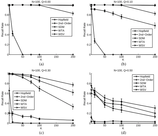
Second, the number of neurons in the network (N) is set to 100 and the number of fundamental vectors (K) is varied from 10 to 200. For comparisons, we implemented the Hopfield network, second order memory and SDM, and tested them under the same condition with our approximation models. The number of addresses in SDM is set to N2 to make the storage requirements comparable to our models. The select radius of SDM is set using the formula described in Section II-B.
The results are shown in Figure 4. Due to its limited capacity, the performance of the Hopfield network is low compared to others. SDM performs well when no noise is present to a probe vector; The recall rate is the highest whenN ≤50and comparable to that of the second order memory for N > 50. However, it does not retain the performance as Q increases. The performance of WSV is consistently better than that of the WTA, except for
Q= 0.5andK <50. The performance of WSV model is highly comparable to the second order model forK≤N. Although the second order model retains high recall rates asK becomes more thanN, both WTA and WSV fail to do so. The results suggest that the approximation models are capable of storing patterns as many asN.
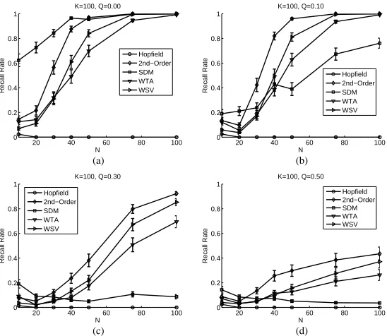
Next, K is fixed to 100, and N is varied from 10 to 100. The results are shown in Figure 5. Observations similar to ones for Figure 4 can be made. When there is no noise in a probe vector, SDM has the highest recall rate of close to 100%. The performance degrades quickly as noise is being introduced. Recall rates of the Hopfield network are consistently low due to its limited capacity. The performance of WSV is consistently better than that of WTA, except forN <50. The performance of WSV is comparable with the second order model when Q≤0.1
andN ≈K.
Some descriptive statistics of mean recall rates normal-ized by corresponding mean recall rates of the second order memory are shown in Table I. The normalized mean recall rate is 1.0 if the mean recall rate is the same with that of the second order memory and less than 1 if it is less than that of the second order memory. Shown in the table are the mean, median, first quartile (1st Q), third quartile (3rd Q), and standard deviation (Std). The mean of SDM is deceptively high because of a few entries that are more than 3. Overall, the proposed approximation models are most comparable to the performance of the second order memory. The results also suggest better and more stable performance of the weighted significant voting than the winner-take-all model.
V. ARCHITECTURE
(b)
20 40 60 80 100
0 0.2 0.4 0.6 0.8 1
N
Recall Rate
K=100, Q=0.10
theta=1.50 theta=1.75 theta=2.00 theta=2.25 theta=2.50 theta=2.75 theta=3.00 theta=3.25
20 40 60 80 100
0 0.2 0.4 0.6 0.8 1
N
Recall Rate
K=100, Q=0.30
theta=1.50 theta=1.75 theta=2.00 theta=2.25 theta=2.50 theta=2.75 theta=3.00 theta=3.25
20 40 60 80 100
0 0.1 0.2 0.3 0.4 0.5
N
Recall Rate
K=100, Q=0.50
theta=1.50 theta=1.75 theta=2.00 theta=2.25 theta=2.50 theta=2.75 theta=3.00 theta=3.25
(a)
(c) (d)
20 40 60 80 100
0 0.2 0.4 0.6 0.8 1
N
Recall Rate
K=100, Q=0.00
theta=1.50 theta=1.75 theta=2.00 theta=2.25 theta=2.50 theta=2.75 theta=3.00 theta=3.25
Figure 3. Comparing memory recall rates of the Weighted Significant Voting with variousθs.
(b)
50 100 150 200
0 0.2 0.4 0.6 0.8 1
K
Recall Rate
N=100, Q=0.10
Hopfield 2nd−Order SDM WTA WSV
50 100 150 200
0 0.2 0.4 0.6 0.8 1
K
Recall Rate
N=100, Q=0.30
Hopfield 2nd−Order SDM WTA WSV
50 100 150 200
0 0.2 0.4 0.6 0.8 1
K
Recall Rate
N=100, Q=0.50
Hopfield 2nd−Order SDM WTA WSV
(a)
(c) (d)
50 100 150 200
0 0.2 0.4 0.6 0.8 1
K
Recall Rate
N=100, Q=0.00
Hopfield 2nd−Order SDM WTA WSV
Figure 4. Comparing memory recall rates withN= 100and variousK.
TABLE I.
DESCRIPTIVE STATISTICS OF THE NORMALIZED MEAN RECALL
RATE.
Method Mean Median 1st Q 3rd Q Std Hopfield 0.09 0.00 0.00 0.00 0.226
SDM 0.834 0.686 0.138 1.00 0.870 WTA 0.751 0.782 0.550 0.992 0.238 WSV 0.764 0.850 0.531 0.987 0.232
One subtle but critical issue to the designs is the semantic of a bit signal. We want to allocate a single bit to encode the state of a single memory cell (xij), which
is bipolar (±1). However, most conventional computing platforms use the binary representation (0/1). To utilize the rich existing computing conventions, therefore, the bipolar signals need to be converted into the binary rep-resentations internally. Fortunately, all designs considered in this section interface the state vector (x) with either bit-word or bit-bit multiply-accumulator (MAC), and we can build-in the bipolar-binary conversion into the MAC with little overhead. More details of MAC designs are given below.
(b)
20 40 60 80 100
0 0.2 0.4 0.6 0.8 1
N
Recall Rate
K=100, Q=0.10
Hopfield 2nd−Order SDM WTA WSV
20 40 60 80 100
0 0.2 0.4 0.6 0.8 1
N
Recall Rate
K=100, Q=0.30
Hopfield 2nd−Order SDM WTA WSV
20 40 60 80 100
0 0.2 0.4 0.6 0.8 1
N
Recall Rate
K=100, Q=0.50
Hopfield 2nd−Order SDM WTA WSV
(a)
(c) (d)
20 40 60 80 100
0 0.2 0.4 0.6 0.8 1
N
Recall Rate
K=100, Q=0.00
Hopfield 2nd−Order SDM WTA WSV
Figure 5. Comparing memory recall rates withK= 100and variousN.
signal is interpreted as bipolar, the arrow accompanies a small line segment perpendicular to the arrow. A multi-bit signal is shown by a black arrow. A vector signal carrying number of either bit or multi-bit signals is shown by a thick arrow. The shade of the thick arrow is dependent on the type of the signal. A bit vector signal is in gray, a multi-bit vector signal is in black. For our discussion, we assume that eigenvalues and eigenvectors of the decomposition (11) are represented with L-bits multi-bit signals. Figure 6 shows the different kinds of arrows used in this section.
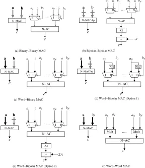
The designs deploy a number of multiply-accumulate (MAC) units which computes an inner product of two vectors. Figure 7 shows five different types of MAC units used in our designs. Each type is shown its block representation (left) and architectural-level design (right). Figure 7(a) shows a binary-binary MAC, where both inputs are binary vector signals. It can be implemented withNmultiplexers and oneN-input accumulator (shown as N-AC in the figure). The accumulator can be built with
N−1 adders of at mostlog2N bits. It does not require any multipliers, thus can be implemented inexpensively. Figure 7(b) shows a bipolar-bipolar MAC where both inputs are bipolar vector signals. As for the binary-binary MAC, it can be implemented withNmultiplexers and one
N-input accumulator. However, in this case, the output of the accumulator needs to be multiplied by 2 and then subtracted by N. This arithmetic implements a binary-bipolar conversion.
Figure 7(c) shows a word-binary MAC, which takes one multi-bit vector and one binary vector. Like the binary-binary MAC, it requires N multiplexers and an
N-input accumulator, but does not require multipliers. The N-input accumulator is more expensive than that of Figure 7(a) and (b) as additions involve at mostLlog2N
(c) Binary vector signal
(d) Bipolar vector signal (f) Multi−bit vector signal (a) Binary signal
(e) Multi−bit signal (b) Bipolar signal
Figure 6. Different signal types and corresponding arrow representa-tions.
bits.
Figure 7(d) shows a word-bipolar MAC, which takes one multi-bit vector and one bipolar vector. It is similar to the word-binary MAC of Figure 7(c) except that the inputs to multiplexers are the multi-bit input and its negative. For a sign-magnitude format, computing the negative of a multi-bit number is as simple as to invert the sign bit. For a 2’s complement number, it is to take the 2’s complement. When the multi-bit vector is fixed, we can employ an alternative approach, which can reduce the implementation cost for a largeN. This alternate scheme is shown in Figure 7(e). Instead of computing the negative of each multi-bit number, it converts a word-binary MAC to a word-bipolar MAC using a similar strategy with the bipolar-bipolar MAC of Figure 7(b). In our designs, we employ this alternative approach in implementing word-bipolar MACs.
Finally, Figure 7(d) shows a word-word MAC, which takes two multi-bit vectors as inputs. It requires N L -bit multipliers and one N-input 2Llog2Naccumulator.
Therefore, it is considerably more expensive than the other two.
A. Second-Order Model
bN
1 0
aN bN
N−AC 1 0
b1
a1 a1
X2 1 0
aN bN
N−AC 1 0
b1
Σa i
bN b1
a1 0 aN
N−AC
1 0
aN bN
N−AC 1 0
b1
aN
N−AC
b1 bN
Mult Mult
X2
...
N−AC
1 0 1 0
(b) Bipolar−Bipolar MAC
c
... 1
a
N−MAC/bp
Neg Neg
c (a) Binary−Binary MAC
(c) Word−Binary MAC
0 0
(d) Word−Bipolar MAC (Option 1)
+
c ...
0 0
1
a
(f) Word−Word MAC (e) Word−Bipolar MAC (Option 2)
c ...
1 0 1 0
0
N−MAC a
c
c
c N−MAC
c N−MAC
c
... 0 0
1
a
a
c N−MAC/bp
N−MAC
c
1
a
...
+ −N
c
b b
b
a a b
b a b
b
a
1
Figure 7. Various types of multiply-accumulate units used in the memory designs.
of Equation (12). Figure 2 shows its architectural-level design of the ith memory cell.
The jth neuron (Φij) in the first layer computes a dot-product between x andvij to compute the unit response. The output ofΦij is delivered to the second layer neuron via an L-bit bus. The second layer neuron (Ψi) first squares each input and takes a dot-product between the squared inputs andλi= [λi1, λi2, ..., λiR].
B. Sparse Distributive Memory Model
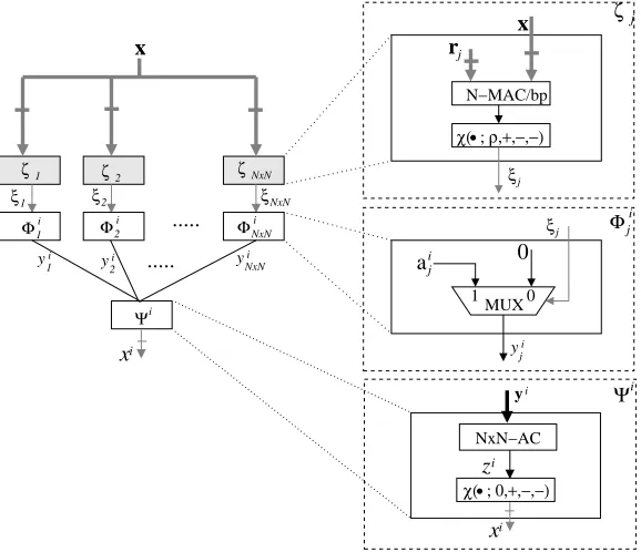
Next model to be considered is the Sparse Distributive Memory (SDM). Figure 9 shows its architectural-level design of the ith memory cell. The architecture departs slightly from the two-layered one shown in Figure 2. It requires an additional layer at the very front as indicated with a set of shaded blocks (η·s). We call this layer the address layer, as it implements the address block of the memory. The address layer is shared among all memory cells in the memory. Each neuron in the address layer computes a dot-product between x and a random vector (rj) associated with the neuron. The result of the dot-product is thresholded with the select radius (ρ) to produce a binary signalξj, which is used to activate the
corresponding entry in the content block. See Section II-B for details of the address and content blocks. Note that there are N ×N neurons in the content block as determined in Section IV.
The jth neuron in the first layer (Φij) after the address layer contains a single multiplexer which selects either 0 or the ith entry of the content memory at the j location (aij). It requires at mostlog22Kbits to storeaijasaijcan
take values between[−K, K]. Therefore, we consider the output of Φij to be log22K bit long. Whenξj = 0, 0 is
selected, and whenξj= 1,aijis selected. The output from N×N neurons in the first layer is collected in the second layer neuron,Ψi. It needs to calculate the sum of theN× N numbers, each being log22K bits long. This process requires N×N−1adders of at most 2 log2Nlog22K
bits. The result of the additions is thresholded at 0 to produce the next ith state of the memory.
Costly parts of the design are log2K-bit data-pathes connecting the first layer to the second layer, and theN× N-MAC in Ψi.
C. Winner-Take-All Model
We now consider proposed models to approximate the second order correlation memory. First, we consider WTA. Figure 10 shows an architectural-level design of the model. It obeys the two-layer model of Figure 2 except two one-bit feedback signals (β andγ) from the second to the first layer.
The first layer neurons (Φij) computes a dot-product between
λ
Φi
2
Φi
R
Φi
1
y
i 2y
iR
y
ix
ix
i 1y
iR
y
i ψi jΦi
j
y
i jv
iz
iΨi
z
iχ( ; 0,+,−,+)
x
...
...
x
...
Mult MultN−MAC/bp
R−MAC
i
1
Figure 8. Architectural-level design of the second order correlation memory.
χ( ; ρ,+,−,−) rj
2
ζ ζNxN
Ψi 2
Φi
NxN
Φi 1
Φi 1
ζ
j Φi
j
ζ
zi
y1i y 2
i y
NxN i
yji
χ( ; 0,+,−,−) xi
xi
Ψi ξ1 ξ2
ξj
ξj
ξNxN x
1
0 ...
0
x
ai j ...
NxN−AC
i
y
N−MAC/bp
MUX
Figure 9. Architectural-level design of the sparse distributed memory.
θwhose value is determined in theθ-Adj block shown in Figure 10. When the result of the dot-product is more than
θ or less than −θ, then the neuron outputs 1. Otherwise it outputs 0. The θ-Adj block implements the following equation.
θ=
⎧ ⎨ ⎩
θ=θ+δ if β= 1 andγ= 0 θ=θ−δ if β= 0 andγ= 0
θ=θ0 if γ= 1
, (33)
δ=
δ/2 ifγ= 0
θ0/2 ifγ= 1 . (34)
Thus, the block can be implemented with an adder and either a shift register or an adder for computing the division by 2. Note that θ0 is an initial threshold value,
which should be set to k|vjki |
|λij|, the maximum possible value of the dot-product.
The second layer neuron takes a binary vector ofR-bits as the input. The main goal of the neuron is to provide
an R-bit accumulator (shown as R-AC in the figure). The accumulator requiresN−1adders that are at mostlog2R
bits long. Denote the result of the accumulator ci. Then,
ci is passed to both β-Gen block and a comparator (=
1?). Theβ-Gen block basically implements the following equation.
βi=
0 ifci = 0
1 ifci >0 . (35)
The comparator implements the following equation.
γi=
0 if ci= 1
1 if ci= 1 . (36)
Thus,γ1= 1signals that a winner (k˜in Eq. (20)) of the competition is found. The signal is then used to latch the sign of λik˜, which is computed by a dot-product between yi and a vector whosekth entry is the sign ofλik.
The second layer neuron requires, therefore, two com-parators (one for detectingci= 0and the other detecting
ci= 1), one R-AC whose adders are at mostlog2R bits, one binary-binary R-MAC, and a latch. Communication between first layer and second layer neurons involve only bit signals.
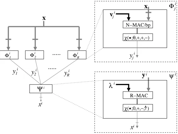
D. Weighted Significant Voting Model
Finally, we consider WSV. It obeys the two-layer network of Figure 2. There are R neurons in the first layer. The jth first layer neuron (Φij) computes a unit response of vij to x using a word-binary N-MAC. The result is thresholded at a pre-defined threshold value ofθ. When the unit response is more than θ or less than−θ, the neuron outputs 1. Otherwise, it outputs 0. The neuron can be completely implemented with one word-binary N-MAC and one threshold logic.
The second layer neuron (Ψi) first computes a dot-product between the input binary vector and λi =
[λi
1, λi2, ..., λiR]. The result is then thresholded at 0. Again,
the neuron can be completely implemented with one word-binary R-MAC and one threshold logic. The com-munication among neurons involves only bit signals.
VI. CONCLUSIONS
The paper introduced two associative memory models that are derived as an approximation to a second order cor-relation model. Both are constructed from an eigenvalue decomposition of a correlation tensor of the second order model. The winner-take-all model selects the eigen-mode with maximum response, while the weighted significant voting selects those that are deemed significant in terms of the unit response. The memory can be implemented with a collection of simple processing units without mul-tipliers, interconnected by a single wire per input/output to transmit its state.
Our numerical experiments suggest better and more stable performance of the weighted significant voting than the winner-take-all model. The design of the weighted sig-nificant voting is simpler than the winner-take-all model, as no feedbacks are necessary. Thus, we can conclude
that the weighted significant voting is preferable to the winner-take-all model for implementing a second order memory.
No theoretical analysis of the approximation models are available at this time. Future works include studying the convergence properties of the models, and deriving the capacity of the models and the size of the attraction basin. With a decent amount of capacity, robustness against noise, and relatively small computational cost, the proposed memory models are valuable alternatives to constructing associative memories.
Another limitation of this study is that it does not consider on-line storage of fundamental vectors. The storage phase is done off-line with a set of fundamental vectors, and eigen-modes are pre-computed and pre-stored in the circuits. For the memory models to become wide-spread use, they needs to be able to update the memory contents with new fundamental vectors with minimum user interactions in a computationally efficient manner.
REFERENCES
[1] T. Kohonen,Associative memory. Berlin: Springer-Verlag, 1977.
[2] M. A. Cohen and S. Grossberg, “Absolute stability of global pattern formation and parallel memory storage by competitive neural networks,” IEEE Transactions on Systems, Man, and Cybernetics, vol. 13, no. 5, pp. 815– 826, Sept./Oct. 1983.
[3] J. J. Hopfield, “Neural nets and physical systems with emergent collective computational properties,” Proceed-ings of the National Acaddemy of Science USA, 1982. [4] V. Gimenez-Martinez, “A modified hopfield
auto-associative memory with improved capacity,” IEEE Transactions on Neural Networks, vol. 11, no. 4, pp. 867–875, 2000.
[5] D. O. Gorodnichy, “The optimal value of self-connection,” in Proceedings International Joint Conference on Neural Networks, Washington DC, July 1999.
[6] O. de Jesus, J. Horn, and M. Hagan, “Analysis of recur-rent network training and suggestions for improvements,” in Proceedings of the International Joint Conference on Neural Networks, Washington, DC, July 2001, pp. 2632– 2637.
[7] Z. Chengxiang, C. Dasgupta, and M. P. Singh, “Retrieval properties of a hopfield model with random asymmetric interactions,”Neural Computation, vol. 12, no. 4, pp. 865– 880, 2000.
[8] D.-L. Lee and T. C. Chuang, “Designing asymmetry hopfield-type associative memory with higher order ham-ming stability,” IEEE Transactions on Neural Networks, vol. 16, no. 6, pp. 1464–1476, November 2005.
[9] W. Krauth and M. Mezard, “Learning algorithms with optimal stability in neural networks,” Journal of Physics A: Mathematical and General, vol. 20, pp. L745–L752, 1987.
[10] S. S. Venkatesh and P. Baldi, “Programmed interactions in higher-order neural networks: The outer-product algo-rithm,”Journal of Complexity, vol. 7, no. 4, pp. 443–479, Dec. 1991.
[11] D. Burshtein, “Long-term attraction in higher order neural networks,”IEEE Transactions on Neural Networks, vol. 9, no. 1, pp. 42–50, Jan. 1998.
R−AC
χ( ;θ,+,+,−)
ij
Φ
i
Ψ 1
Φi
R
Φi
xi 1
yi 2
yi R
yi
xi yi j
yi
i Ψ 2
Φi
βi
vji i
λj
γi β , γi i
β , γi i
β−Gen
ci
ci
... ...
θ−Adj
R−MAC =?1
Latch Load
x
N−MAC/bp x
Sign( )λi
Figure 10. Architectural-level design of the winner-take-all memory.
N−MAC/bp
χ( ;θ,+,+,−)
χ( ;0,+,−, )
i
λ
2
Φi
R
Φi 1
Φi
1
y
i 2y
iR
y
ix
ij
v
ij
Φi
j
y
iψi
x
iy
iΨ
ix
...
...
x
R−MAC
Figure 11. Architectural-level design of the weighted significant voting memory.
[13] U. Bauer, M. Scholz, J. B. Levitt, K. Obermayer, and J. S. Lund, “A biologically-based neural network model for geniculocortical information transfer in the primate visual system,”Vision Research, vol. 39, no. 613-629, 1999. [14] C. Koch,Biophysics of computation. Information
Process-ing in SProcess-ingle Neurons. New York: Oxford University Press, 1999.
[15] T. Kubota, “Second order associative memory models with threshold logics -eigen mode selections,” inProceedings of the IEEE International Conference on Systems, Man, and Cybernetics (SMC), Montreal, Quebec, October 2007, pp. 1884–1889.
[16] L. De Lathauwer, B. D. Moor, and J. Vandewalle, “A multilinear singular value decomposition,” SIAM Journal on Matrix Analysis and Applications, vol. 21, no. 4, pp. 1253–1278, 2000.
[17] J. Bruck and V. P. Roychowdhury, “On the number of spu-rious memories in the hopfield model,”IEEE Transactions on Information Thoery, vol. 36, no. 2, pp. 393–397, 1990.
[18] P. Kanerva,Sparse Distributed Memory. MIT Press, 1988. [19] ——, Associative Neural Memories: Theory and Imple-mentation. New York: Oxford University Press, 1993, ch. 3, pp. 50–76.
[20] T. Fukai and S. Tanaka, “A simple neural network ex-hibiting selective activation of neuronal ensembles: From winner-take-all to winners-share-all,”Neural Computation, vol. 9, no. 1, pp. 77–97, 1997.
[21] Z. H. Mao and S. G. Massaquoi, “Dynamics of winner-take-all competition in recurrent neural networks with lateral inhibition,”IEEE Transactions on Neural Networks, vol. 18, no. 1, pp. 55–69, 2007.
[22] R. P. Lippmann, “An introduction to computing with neural nets,”IEEE ASSP Magazine, Apr. 1987.