Prediction of Temperature Time Series Based on
Wavelet Transform and Support Vector Machine
Xiaohong Liu
Qinggong College, Hebei United University, Tangshan, China Email: [email protected]
Shujuan Yuan and Li Li
Qinggong College, Hebei United University, Tangshan, China Email: [email protected]
Abstract—To predict the time series, a model combining the wavelet transform and support vector machine is set up. First, wavelet transform is applied to decompose the series into sub series with different time scales. Then, the SVM is applied to the sub series to simulate and predict future behavior. And then by the inverse wavelet transform, the series are reconstructed, which is the prediction for the time series. The prediction precision of the new model is higher than that of the SVM model and the artificial neural network model for many processes, such as runoff, precipitation, temperature. And the new Wavelet-SVM model is applied to analyze the month temperature time series of city Tangshan for example. The universal applicability of the new Wavelet-SVM model and the improvement direction are discussed in the end.
Index Terms—Temperature, Regression, Support vector machine, Wavelet Transformation
I. INTRODUCTION
In the time-domain statistical analysis, researchers have paid much attention to empirical risk minimization (ERM) for the past many years. ERM is rational as the empirical risk is approaching the expected risk when number samples are large. However, results based on ERM cannot reduce the real risk in the state of finite samples; that is to say, small training error doesn’t always lead to isound outcome of forecast and simulation. People often refer to the ability of correct prediction using learning machine with the output as generalization ability. In certain cases, the ability to generalize will decline when the training error is too small and the real risk is raised, which is called over fitting [1].That’s because samples are inadequate and the design of learning machine is unreasonable. The two reasons are interrelated. In the neural network, when samples are limited, the learning ability of network is overfit to remember each sample and the empirical risk will quickly converge to a small value or even zero, which cannot guarantee reasonable forecast of future samples. The theory of effective learning and generalizing method needs to be built up under the condition of small samples based on minimizing both empirical risk and fiducially range (VC dimension (VaPnik-Chervonenkis Dimension) of learning machines capacity) because of the contradiction between
complexity and generalization of learning machine, which leads to the production of structure risk minimization (SRM). Actually, support vector machine [2-4] (SVM) is the realization of this theory aimed to pattern recognition.
Compared to traditional neural network [5, 6], SVM method replaces traditional empirical risk with structure risk minimization and solves a quadratic optimization problem which can get the global optimal solution in theory. The method has avoided local extreme value problem in neural network. The theory of support vector machine has become popular since 1990s. The algorithm of SVM is applied to pattern recognition, regression estimate and probability-density function estimate. It is considered as an alternative method of artificial neural network in the classifications of text and recognitions of hand-written character, speech and face because of its excellent performance of study [7, 8].
In recent years, SVM method has been applied to time-series analysis [9-13]. Time-time-series is usually regressed by SVM and then its trend will be predicted in the time-series prediction, which cannot reflect the impact of the blend. However, a lot of time-series are always the superposition of periodic terms and trend terms with the changes of both short-term and long-term characteristics. If the method is used, the impact of short-term will be weakened or even disappears. Wavelet analysis with good time-frequency property just covers the shortage.
Time series are decomposed into different time and scale by wavelet transformation, and thus we can get the property of time series in different frequency bands as time goes by [14]. The method has been widely used in multi-scale analysis of time-series [15-18]. Regularities of short-term (high frequency) and long-term (low frequency) are reflected in different frequency bands after wavelet decomposition of time-series including many process changes by various time scales. If wavelet coefficients in different frequency bands are regressed by SVM, the tendencies of development and the regularities for change of time-series by different time scales will be obtained, which can reflect its natural information better.
time-series will be reconstructed by inverse wavelet transformation. Finally, the changes of time-series in the future will be analyzed and forecast taking the process of temperature for instance.
II. DESIGN OF THE TREND ANALYSIS MODEL FOR THE TIME SERIES BASED ON WAVELET AND SVM
A. Pretreatment of Hydrological time series
At present, wavelet multi-resolution analysis in hydrological process always decomposes original sample data, and then extracts wavelet scale information. This method can reduce time for calculation and simplify calculation process. But there is a problem ignored. In wavelet multi-resolution analysis, what should be decomposed is wavelet coefficient instead of original sample data. Generally, some new information could be obtained by decomposing the original sample directly. However, there is no theoretical support [19].
) (n
x is the direct input to the filter banks, and letxs(t)
is a continuous time function
)
(
)
(
)
(
t
x
n
t
n
x
n
s
where x(n) is the coefficient. Only when ) ( )
(k k
(where
(k) is a sign function), xs(t) has correctcoefficient x(n). Commonly, hydrological time series )
(t
dissatisfy this condition, which is often ignored in wavelet scale analysis for hydrological process. Hence we could construct the known sample x(n)by adjustingthe coefficienta(n), and then we could get a(k) by
)
(
)
(
)
(
t
a
n
t
n
x
n
In fact, time series x(n) is often replaced by
)
(
~
)
(
)
(
n
x
t
t
n
a
t
. (1)Where
~(tn) is the conjugate function of(tn).Then the continuous time function is expressed as followed:
)
(
)
(
)
(
t
a
n
t
n
x
n
s
B. Wavelet transformation and multi-scale decomposition Suppose that (t) is a basic wavelet or mother wavelet.
After translation and dilation for it, the following expression is obtained:
) 0 , , ( 1
) (
,
a R a
a t
a t
a
.
Where,
a
is the dilation factor and
is the translation factor. a,(t) is the mother wavelet depending on parametersa
and
.For any signal f(t) with finite energy, we construct a
continuous wavelet transform (CWT) as follows.
dta t t f a t t f a WT
R a
f
) (), () 1 () ,
( ,
If Csatisfies admissible condition [19] and the signal
) (t
f satisfies the condition
f
(
t
)
dt
Then we can reconstruct f(t) without loss of
information as followed.
0 2
1 ) , ( 1
) (
a da dt a t a a WT C
t
f f
An analysis of a signal based upon the CWT yields a potential wealth of information.The CWT is essentially an exploratory data analysis tool that can help the human eye to pick out features of interest.To go beyond these plots,we are essentially faced with an image processing problem because of the two dimensional nature of the CWT.Since the two dimensional CWT depends on just a one dimensional signal,it is obvious that there is a lot of redundancy in the CWT.For example,there is little difference in the CWT between adjacent scales.We can thus advance beyond the CWT by considering subsamples that retain certain key features.
The Discrete Wavelet Transform (DWT) can be regarded as an attempt to preserve the key features of the CWT in a succinct manner.From this point of view,the DWT can be thought of as a judicious subsampling of
tW
, in which we deal with just ‘dyadic’ scales(i.e.,we pick to be of the form 2j1,j1,2,3,) and
then ,within a given dyadic scale 2j1,we pick times t that are separated by multiples of 2j.Just as a signal
x can be recovered from its CWT, It is possible to recover the data perfectly from its DWT coefficients.Thus ,while subsampling the CWT at just the dyadic scales might seem to be a drastic reduction,a time series and its DWT are actually two representations for the same mathematical entity.
The DWT can be thought as a judicious sub sampling of WTf(a,) in which we just deal with ‘dyadic’ scales
(i.e., we pick
a
to be the form 2 1, 1,2,3,j
j ) and
then, within a given dyadic scale 1
2j , we pick times that are separated by multiples of 2j, namely
k
j
2
;then the wavelet and scaling coefficient of level j is defined as followed,
) mod 1 2 ( , 1 1
0
, 1
j
N l t j L
l l t
j hV
W
) mod 1 2 ( , 1 1
0
, 1
j
N l t j L
l l t
j gV
V
WhereV0X and it represents the initial hydrological time series. t is time, Wj,tis wavelet coefficient of level j of time t ,Vj,tis scaling coefficient of level j of time t,
l l g
h, is equivalent wavelet and scaling filters of level j,
Although in practice Wjand Vjare computed using the pyramid algorithm, it is of theoretical interest to note that we could obtain their elements directly from X via
1 0 mod 1 ) 1 ( 2 , , j j L l N l t l j tj h X
W
1 0 mod 1 ) 1 ( 2 , , j j L l N l t l j tj g X
V
Where
hj,l and
gj,l are the jth level equivalentwavelet and scaling filters,each having width
2 1
1
1 L
L j
jj
Here h1,l hl and g1,l gl ,these filters have transfer
functions
2 0 1 2 2 j l l jj f H f G f
H
1 0 2 j l lj f G f
G
Again, H1
f H
f and G1
f G
f . The filter
hj,l is nominally a band-pass filter with pass-bandgiven by j j
f 1/2 2
/
1 1 , where
l j
g , is nominally a low-pass filter with pass-band 1
2 / 1
0 f j
Given Wjand Vj, we can reconstruct the elements of
1
j
V via the jth stage of the inverse pyramid algorithm, namely,
1 0 mod , 1 0 mod , ,1 1 1
L l N l t j l L l N l t j l t
j hW j gV j V , 1 , , 1 ,
0 1
Nj
t where
1 , , 3 , 1 , 2 , , 2 , 0 , 0 1 2 1 , 1 , j t j j t
j W t N
N t W t j
V , is defined similarly. The procedure of inserting a single zero between the elements of
Wj,t to form
t j
W, is called ‘up sampling by two’.
If W, V represents the DWT wavelet and scaling coefficients respectively, then the following functions can be derived.
PX
W
, V QXWhere P is a NNreal matrix and satisfiesPTPIN, so we could reconstruct the expression of X.
J J j j J T J J j j T
j W Q V D S
P
X
1 1
Each Dj is a time series related to variations in X at the scale of j
2 . In a multi resolution analysis,Dj is called the wavelet detail of level j, and
J J
j k
k
j D S
S
1
is
called the wavelet smooth of level j for X. The wavelet detail reflects the detail variations on different time scales, and the wavelet smooth reflects the general trend on different time scales.
From the decomposition process above, original time series are decomposed to different scales. On one hand, long-term change process of series can be observed and analyzed; on the other hand, information about short-term series change and the singularity of the time series can be obtained.
C. Support Vector Machine Regression and predication Calculate the regression function through the support vectors using the obtained coefficient, and then forecast the trend change of the future. The basic idea of support vector machine regression is nonlinear mapping the original data x into its high dimensional feature space.
Make
n i i i ax
G , 1 a given training data set (
x
iisthe input vector,
a
iis the observed value and n is the total number of data). The form of SVM decision function is as following.b x
f
( i) (2)Where,
(xi)is the non-linear mapping turning inputvectors into high dimensional feature space. The coefficients
andb
are estimated by minimizing the regularized risk function
N i i i f a C f r 1 2 2 1 ) , ( )( (3)
The first term is the empirical error (risk); the second term 2
2
1 is a measure of the flatness of the function. C is the regularized constant determining the tradeoff between the empirical risk and the flatness of the model.
) , (ai fi
is called loss function. Among loss functions
-insensitive function [20] is most widely used, and it takes the following form.
Ni i i
i i i i otherwise f a f a f a 1 0 ) , (
(4)
is called tube size and the
-insensitive function doesn’t penalize the error below
. The smaller is
and the higher is the approximation accuracy placed on the training data. C and
are both user-defined parameters.By introducing positive slack variables
and
, Eq. (3) is transformed to the following primal problem. Min
N
i i i C r 1 2 ) , ( 2 1 ) , ,
( (5) s.t. : N i a b
xi) i , 1,2, ,
( N i b x
ai
( i)
i, 1,2,,N i
i
i, 0, 1,2,,
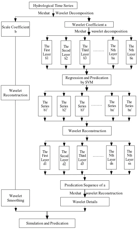
wavelet Reconstruction wavelet decomposition Wavelet Decomposition
Mexhat
Hydrological Time Series
Scale Coefficient b
Wavelet Coefficient a
Regression and Predication by SVM The First Layer b1 Wavelet Reconstruction
Predication Sequence of a
Wavelet Details
Simulation and Predication Mexhat The Secod Layer b2 The Third Layer b3 The Nth Layer bn The Nth Layer bn The Series b1′ The Series b2′ The Series b3′ The Series bn′ The Series bn′ The First Layer d1 The Secod Layer d2 The Third Layer d3 The Nth Layer dn The Nth Layer sn Mexhat Wavelet Reconstruction Wavelet Smoothing
Figure 1. The calculation steps based on Wavelet-SVM model
N i i i i i N i i i i i N i N i i i i i i i b x a a b x C b L 1 * * 1 1 1 2 ) ( ) ) ( ( ) ) ( ( ) ( 2 1 ) , , , , , , , ( (6) And the following functions can be deduced according to extreme conditions.
n i i i i x L 1 0 ) ( ) ( (7)
n i i i b L 1 0 )( (8)
0 i i i C
L
( 9 )
0
i i
i
C
L
(10)Next, Karush-Kuhn-Tucker condition is applied to regression, and the conjugate Lagrangian function (11) is deduced when the expressions of (7) and (10) are applied in function (5).
N i N i i i i i i j i j j n i n j ii x x
L 1 1 1 1 ) ( ) ( ) ( ) ( ) )( ( 2 1 (11)
So, whenK(xi,xj)equals to(xi)(xj), the conjugate
Lagrangian function (11) can be obtained. Min ) , ( ) )( ( 2 1 ) ( ) ( ) , ( 1 1 1 1 j i j j N i N j i i n i i i n i i i i i i x x K
(12) s.t. : 0 , , 2 , 1 , 0 , , 2 , 1 , 0 0 ) ( 1
i i i i n i i i N i C N i C Calculate value of
iand i
, the optimal weight of vector of regression hyperplane is as following.
i ni
i
i
x
1 (13)Finally, when the above expressions are applied to the function (2), the regression function can be obtained and it is as follows.
n
i
i i i
i K x x b
x g 1 ) , ( ) ( ) , ,
( (14) where K(xi,xi) is called kernel function. The value of
the kernel equals to the inner product of two vectors of
) (xi
and
~(xi) in the feature space. Namely, ) ( ~ ) ( ) ,(xi xi xi xi
K
. Any function satisfying Mercer condition can be named kernel function [21].After the regression function is derived, the scale of temperature prediction time is inputted, the prediction is obtained corresponding to the wavelet coefficient.
D Wavelet Reconstruction
By using support vector regression, the prediction data is obtained corresponding to the wavelet coefficient, and then
a
n is reconstructed.E. Post-treatment
In section above, we reconstruct
a
n , which is the wavelet coefficient instead of the real prediction data.According to
n
s
t
a
n
t
n
x
(
)
(
)
(
)
, filter again, and then we’ll get the real prediction data.F. The calculation steps of the Wavelet-SVM model based on MEXHAT wavelet
wavelet analyses of actual time series. Generally speaking, our choice is dictated by a desire to balance two considerations. On the one hand, wavelet filters of the very shortest widths can sometimes introduce undesirable artifacts into the resulting analyses. On the other hand, while wavelet filters with a large L can be a better match to the characteristic features in a time series, their use can result in (i) more coefficients being unduly influenced by boundary conditions, (ii) some decrease in the degree of localization of the DWT coefficients and (iii) an increase in computational burden. A reasonable overall strategy is thus to use the smallest L that gives reasonable results. Based on literature [19], the Mexican hat wavelet is selected. And the calculation steps is shown as followed in Figure 1.
III. CASE STUDY
A. Background
We choose the data of temperature of City Tangshan from 1960 to 2010. In this paper, the monthly temperature from 1960 to 2007 is used as training samples for parameters estimating, and the monthly temperature from 2008 to 2010 is chosen for testing samples. The result obtained from the model is compared to actual temperature volume, and precision of the model is analyzed and tested.
B. Data Preprocessing
Described by above, the data are preprocessed by MEXHAT wavelet before multi-level decomposition. We can get the wavelet coefficients required according to
n
k
n
n
x
k
a
(
)
(
)
~
(
)
.The processed data are shown in figure 2.
Figure 2. Wavelet coefficients obtained from Mexhat process
Shown in Figure 2, preprocessed wavelet coefficients are quite different from the original data and they cannot be simply equaled. As a result, data preprocessing of hydrological is necessary.
C. Multi-level decomposition of wavelet
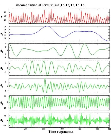
We make a multi-level decomposition of preprocessed wavelet coefficients, which is shown in Figure 3.
Figure 3. The results of wavelet decomposition
Shown in Figure 3, the original signal is superimposed by many different periodic signals. Various periodic signals are fully displayed after multi-level decomposition and each time scale reflects corresponding periodic signal. Level-D2 decomposition reflects the periodic change of monthly in different years. The original signal is decomposed into different frequencies, which is more conducive for modeling and accurate prediction.
D.Prediction based on support vector machine
All levels signals received by decomposition are learned and trained by support vector machine. During the process, selection of kernel function is important. The common kernel functions are radial basis function, polynomial kernel function, Cauchy function [21] and so on. Here, the radial basis function is selected to establish the experimental model. Its form is as follows:
TABLE I
THE RESULTS OF PARAMETERS OF OPTIMIZATION BASED ON SVM
Band of
regression
ε
CNumber of support vector
a5 0.55 0. 50 10 3
d5 0.55 0.50 20 3
d4 0.05 0.35 15 11
d3 0.23 0.35 15 15
d2 0.55 0.25 15 20
Figure 4. The predicting results of each level wavelet based on SVM in the years from 2008 to 2010
Figure 5. Note how the caption is centered in the column.
2
2
2 exp ,
i i
x x x
x K
So far, the selections of parameter
, (Shown in Formula 4)
and C (Shown in Formula 3&4) based on SVM have lacked the supports of specific theories. According to experience, attempts are often used. In the practical applications, the value of
is less than 2; the value of
is between 0 and 1, chosen less than 0.5; the selection of value of C is more flexible and its range is between 0 and 100. In this paper, the wavelet coefficient on each frequency band and the scale factor on 5th floor shown in Figure 4 are trained respectively. The corresponding parameters of optimization are shown in the table I.Each frequency band is regressed by SVM using the parameters above and the trend of the next three years is predicted. The results are shown in Figure 4.
According to Figure 4, different cycles and trends from the forecast of temperature sequences are shown on various frequency bands. These complex components reflect the master of regularity for the series on different bands, which produces the temperature sequences. The properties on each band are used for the prediction of temperature sequences, which is of advantage to discover the essential regularity.
E. Wavelet reconstruction and post-processing
The forecasting sequences shown in Figure 4 are reconstructed. And
a
(
n
)
is obtained from the formula (1). The results of monthly temperature forecasts among the years of 2008 to 2010 based on)
(
)
(
)
(
t
a
n
t
n
x
n
s
are shown in Figure 5.
According to Figure 5, wavelet model based on SVM
has almost captured the regularity of temperature changes of City Tangshan. The temperature has been predicted accurately in 24 months except the 21th month for the first two years. Although the prediction error increases in the third year, the trend of temperature is still accurate.
F. Analysis and comparison of predicted results
The results of prediction based on single SVM and BP neural network are also shown in order to compare the merits of three methods. Mean square error (MSE) and average relative error
y
ˆ
are taken as the evaluation basis of predicted results to evaluate the forecast accuracies of three methods quantitatively [22], where
i
i i y
y n y
MSE ˆ 1 ( ˆ)2
i i i i
y y y n yˆ 1 ˆ
.
i
y
ˆ
represents the observed annual temperature andi
Figure 6. The comparison of actual data with the prediction based on SVM and BP
As is shown in Table II, method applied in this paper is obviously better than the methods based on single SVM or BP neural network.
In order to compare the merits of three methods clearly and directly, the results obtained from the methods based on single SVM or BP neural network are shown in Figure 6.
According to Figure 6, the accuracies of forecasting based on single SVM and BP neural network are not high. In the first year, the months of inaccuracy results based on SVM are April, May, July and September, and the error based on BP neural network is greater. In the third year (2010), the trend of prediction obtained from SVM is rough, and the trend based on BP neural network cannot be seen at all. It indicates that the methods based on SVM and BP neural network are not good at getting information from original data. They are suitable for short-term forecast of one year and need to be improved further.
The method of wavelet based on SVM is better than the methods based on single SVM and BP neural network both on the precision of prediction and the length of time, which is shown in Figure 6.
IV. CONCLUSION AND DISCUSSION
Different scales of some time series are reflected on different frequency bands. Therefore it is not rigorous to predict the trend in the future using SVM regression this processes. The regression on Wavelet coefficients based on SVM on different scales on time series is presented, which gives full consideration of the impact of regularity for series on various scales and frequencies. The shortcoming of high frequency part (short period) weakened by SVM has been overcome. The problem caused by the continuous wavelet transform in the discrete time-series has been solved through the wavelet transform. The monthly temperature time-series data from city Tangshan is applied to the model as an example. The result indicates that the accuracy obtained from SVM method based on wavelet transform is significantly higher than that based on SVM and BP models.
The method based on wavelet-SVM can dig up deeper information contained in the process of time-series and produce better results of prediction. The method could be applied to many processes, such as precipitation ,runoff and so on.
Trial is used for the selection of the SVM parameters and the number of input parameters for SVM training and predicting. Selection of parameters is an important part of the model building. How to choose suitable parameters need further study. Besides, the paper only takes the radial basis function as kernel function for study. Different kernel function has direct impacts on the establishment of SVM model. For this reason, choosing other types of kernel function for comparative research is worth discussing deeply.
REFERENCES
[1] Zaoqi Bian, Xuegong Zhang. Pattern Recognition
[M].Beijing: Tsinghua university press. 1999.12.
[2] Vladimir N, Vapinik. Statistical Learning Theory, Wiley-Interscience, 1998.
[3] Nello Cristianini, John Shawe-Taylor. An Introduction to Support Vector Machines and other Kernel-based Learning Methods. Cambridge University Press, 2000.
[4] XU Jianhua, ZHANG Xuegong, LI Yanda. Advances in Support Vector Machines. Control and Decision. 2004, 19(5):481-484.
[5] JIN Long, QING Weiliang. A Multi-Step Prediction Model of Wavelet Neural Network. Scientia Atmospheric Sinica.2000,24(1):79-86.
[6] CHEN Renfang, LIU Jing. The Area Rainfall Prediction of Up-river Valleys in Yangtze River Basin on Artificial Neural Network Modes. Scientia Meteorologica Sinica, 2009, 24(4): 483-486.
[7] Jonsson K, Matas J, Kittler J and Li Y P. Learning Support Vector Machines for Face Verification and Recognition. In Proc, IEEE Intl. Conf. Automatic Face and Gesture Recognition, pages 208-213,2000
[8] Byun H, Lee S, W. Applications of Support Vector Machines for Pattern Recognition: A Survey [A].In: Proceeding of the First International Workshop on Pattern
Recognition with Support Machines [C].Niagara
Falls,2010:213-236
[9] Shivam Tripathi, Srinivas V V, Ravi S. Nanjundiah. Downscaling of Precipitation for Climate Change Scenarios: A Support Vector Machine Approach, Journal of Hydrology, 2009.04
TABLE II.
THE ERROR COMPARISON OF MONTHLY TEMPERATURE PREDICTION FROM SANMENXIA GAUGING STATION FROM 2008 TO 2010
Year
Wavelet based on SVM
SVM BP neural
network
MSE
2008 0.0937 0.5451 1.0076
2009 0.2999 1.0772 1.3216
2010 0.5524 1.4824 2.4541
2008 2009 0.0211 0.0360 0.1132 0.1515 0.2021 0.2232[10]Wei-Chiang Hong, Ping-Feng Pai. Potential Assessment of the Support Vector Regression Technique in Rainfall Forecasting, Water Resource Manage, 2006 DOI 10.1007/s11269-006-9026-2
[11]LIN Jianyi, CHENG Chuntian. Application of Support Vector Machine Method to Long-term Runoff Forecast. Journal of Hydraulic Engineering.2010,37(6):681-686. [12]JianDing Qiu,Sanhua Luo,Jianhua Huang. Prediction
Subcellular Location of Apoptosis Proteins Based on Wavelet Transform and Support Vector Machine. AMINO
ACIDS Volume 38,Number 4,1201-1208, DOI:
10.1007/s00726-009-0331-y.
[13]Chun Liu, Changssheng Xie, Guangxi Zhu and Qingdong Wang Obscene. Picture Identification Based on Wavelet Transform and Support Vector Machine. Advanced Research on Computer Education, Simulation and Modeling. Communications in Computer and Information Science, 2011, Volume 176, 161-166, DOI: 10.1007/978-3-642-21802-6_26.
[14]Gilbert String, Truong Nguyen. Wavelets and Filter Banks, Wellesley College, 1996
[15]SHAO Xiaomei, XU Yueqing, YAN Changrong.Wavelet Analysis of Rainfall Variation in the Yellow River Basin. Acta Scicentiarum Naturalium Universitatis Pekinesis. 2006, 42(4): 503-509.
[16]FENG Jianmin, LIANG Xu, ZHANG Zhi, et al. Analysis on Multi-scale Features of Precipitation in East and Middle Part of Northwest China and West Mongloia. Scientia Meteorologica Sinica.2005, 25(5): 474-482.
[17]XU Yueqing, LI Shuang Cheng, CAI Yunlong. The Study
on the Precipitation of Heibei Plain Based on Wavelet Analysis. Science in China, Ser. D. 2004,3 4(12): 1176-1183.
[18]YAO Jianqun. Continuous Wavelet Transforms and Their Applications to Surface Air Temperature and Yearly Precipitation Variations in Yunnan During Last One Hundred Years. PLATEAU METEOROLOGY. 2001, 02: 20-24.
[19]Wang H R, Ye L T, Liu C M, et al. Problems Existing in Wavelet Analysis of Hydrologic Series and some Improvement Suggestions [J]. Progress in Natural Science, 2007, 17(1): 80-86.
[20]SeholkoPfB, Simard P.Smola A J. Prior. Knowledge in SuPPort Vector Kernels [C]. Advanced in Neural Information Processing Systems. MA: MIT Press, 1998. 640-646.
[21]Smits G F, Jordnaa E M. Improved SVM Regression Using Mixtures of Kemels [A]. Proceedings of the 2002 International Joint Conference on Neural Networks[C]. Hawaii: IEEE, 2008. 2785-2790.
[22]Wang Songgui. Linear Models Introduction [M]. Beijing: science press, 2004, 05.
Xiaohong Liu was born in Tangshan, HeiBei province, china, in 1976. She graduated from Beijing Normal University, got the master of Science degree at the same school. And the major field of study was mathematical Statistics and the application of wavelet transform.
She has been a secondary school teacher for seven years. After graduated from Beijing Normal University, she became a lecturer in department of Qinggong College, Hebei United University.
Shujuan Yuan was born in Tangshan, September, 1980, Received M.S. degree in 2007 from School of Sciences, Hebei University of Technology, Tianjin, China. Current research interests include integral systems and computational geometry. She is a lecturer in department of Qinggong College, Hebei United University