Research on the Dynamic Relationship between Prices of Agricultural Futures in China and Japan

Research on the Dynamic Relationship between

Prices of Agricultural Futures in China and Japan

Qizhi HE

School of Finance, Anhui University of Finance and Economics, Bengbu 233030, China Email: happyhefei2000@qq.com

Abstract—Based on the classical regression model,

time-varying coefficient model, unit root, co-integration, Granger causality test, VAR, impulse response and variance decomposition, the dynamic relationship between prices of natural rubber futures in China and Japan has been researched systematically. The following conclusions are gotten through empirical researches: Firstly, there is a stable co-integration relationship between prices of natural rubber futures in China and Japan. Secondly, the time-varying coefficient model is superior to the classical regression model. The influence of price of natural rubber futures in Japan on price of natural rubber futures in China is time-varying. In the long run, the impact of natural rubber futures in Japan on natural rubber futures in China has been gradually increased. Thirdly, the influence of price of natural rubber futures in Japan on price in China is greater than the influence of price in China on price in Japan.

Index Terms—futures, price, time-varying coefficient model,

co-integration

I. INTRODUCTION

Because the natural rubber has excellent physical and chemical properties, so it has a wide range of uses, and there are about more than 70,000 kinds of items which are made partially or completely of natural rubber. From the supply side, China is one of the main origins of natural rubber in the world. From the demand side, China is one of the most important consumers of natural rubber in the world (Shanghai Futures Exchange, Trading Manual for contracts of Natural rubber futures, and 2008 Edition) [1].

With the integration of world economy and the deepening of Chinese openness, the relationship between Chinese economy and the other foreign economy has become more closely. In particular, China has joined the World Trade Organization, and will gradually follow the relevant World Trade Organization agreement. The price dependence of commodities at home and abroad has become higher and higher. In recent years, China's consumption of natural rubber is increasingly dependent on imports. With the continuous deepening and promotion of China's opening up, and china’s continuing to honor commitments on the WTO after China's accession to WTO, the demand of China, gradually as the "World Factory", for natural rubber will continue to increase and in later years China will be increasingly

dependent on imported natural rubber. (Shanghai Futures Exchange, Trading Manual for contracts of Natural rubber futures, 2008 Edition)[1].Thus, the trend of natural rubber futures prices and the dynamic dependencies between China and other major overseas markets have strategic importance. All this need us to study the dynamic trends of prices of China's natural rubber futures at an international perspective.

At presently, Japan's Tokyo Commodity Exchange (TOCOM) and Osaka Mercantile Exchange (OME), China's Shanghai Futures Exchange (SHFE), Singapore Commodity Exchange Limited (SICOM), and etc are the main international trading site for natural rubber futures. Many scholars’ empirical studies show that there are a certain dynamic dependencies and linkages between these cross-rubber future markets. A significant change of a country's rubber future price often gives impact to other country's rubber future prices and lead to changes of other country's rubber future prices. In the international exchange markets of natural rubber futures, the exchange markets in Japan account for a large market share and have great influence on other exchange markets, and transactions in Japan can basically reflects the situation of world market prices of natural rubber futures. (Shanghai Futures Exchange, Trading Manual for contracts of Natural rubber futures, 2008 Edition; Analysis on the main factors which influence the price volatility of China rubber futures, China rubber)[1, 2].

In general, with the development of reform and opening up and the integration of the world economy, the link between the natural rubber futures markets at home and abroad is increasingly interconnected, and the prices and yields of China's natural rubber futures are more and more dependent on those of a number of major international rubber futures market. Natural rubber futures market in Japan (Japan's TOCOM and OME) is one of the most representatives of the international markets of natural rubber futures markets, Therefore, the paper study systematically the dynamic dependency and linkage effect between the natural rubber futures markets in China and Japan.

II. LITERATURE REVIEW

and others. RENHAI HUA and BAIZHU CHEN (2004) [3] studied empirically the dynamic relationship between the domestic and foreign futures prices (Copper, aluminum, soybean and wheat). JIN Tao, Miao Baiqi, HUI Jun (2005) [4]examined empirically the dynamic relationship of march copper futures prices between the Shanghai Futures Exchange and the London Metal Exchange by use of the casual relationship model. Zhao Liang and Liu Liya (2006) [5] studied the relationship between copper future prices of the Shanghai Futures Exchange and the London Metal Exchange using cointegration and Granger Causality Test. LIU Qing-fu, ZHANG Jin-qing, HUA Ren-hai (2008) [6] studied empirically the causal relationship between metals futures (copper futures and aluminum futures) prices of the Shanghai Futures Exchange and the London Metal Exchange by building some kind of model. However, there is still relatively little research on natural rubber futures. In fact, it has important theoretical and practical significance to research natural rubber, because natural rubber belongs to agricultural products futures at the angle of its source, but if seen from the wide range of industrial uses, natural rubber also belongs to industrial products futures.

At the same time researches on the relationship between the futures markets at home and abroad are mainly confined to the traditional constant coefficient regression model. In fact, as for changes of global and regional economic environment, world political situation, government intervention, transaction costs and exchange rates, and frequent occurrences of climate and other natural disasters, changes of domestic and international futures markets are non-symmetrical, and their relationship is also time varying. Thus the traditional constant coefficient regression model can not fully and accurately measure the dynamic relationship between domestic and foreign futures markets. It is more suitable to the actual market situation for the paper to measure dynamically the relationship between the futures markets at home and abroad by use of the time-varying coefficient model. In addition, the paper study dynamically the relationship between the futures markets at home and abroad based on other methods such as Granger causality test, VAR, impulse response and variance decomposition. In a word, the paper has important theoretical and practical significance.

The following parts of this paper are organized as follows: First of all is to introduce some of the econometric model and method, which will be used in the later empirical study, such as time-varying coefficient model, unit root, cointegration, Granger causality test, VAR, impulse response, variance decomposition and etc. Then, using the method described above, the empirical study on the dynamic relationship between Chinese natural rubber futures price series and Japanese rubber futures price series is carried out. The last part is the conclusions which summarize the results of empirical research and gives some suggestions.

III. THE MODEL INTRODUCED

A. The Time-Varying Coefficients Model of the Relationship between Futures Prices at Home and Abroad

In order to measure dynamically the long-term relationship between Chinese and Japanese rubber futures prices, we construct the time-varying coefficients model of the relationship between Chinese and Japanese rubber futures prices based on the time-varying coefficients model (E. SCHLICHT (1989) [7]; E. SCHLICHT (2005)).

1 2

(ln )

C

_t

=

a

_t

+

a

_t

(ln )

J

_t

+

u

_t

(1)

1 1 1 1

2 2 1 2

t t t

t t t

a a v

a a v

− −

⎛ ⎞ ⎛ ⎞ ⎛ ⎞

= +

⎜ ⎟ ⎜ ⎟ ⎜ ⎟

⎝ ⎠ ⎝ ⎠ ⎝ ⎠ (2)

Where

(ln )

C

_t is the dependent variable which

represents Chinese rubber futures price.

(ln )

J

_t is the independent variable which represents Japanese rubber futures price.

(

a

1t

,

a

2t

)

'

is the coefficient vector, and

the disturbance terms,

u

_t∼_N(0,

σ

2_)，

1t

v

∼ 2

1

(0, )

N σ ，

2t

v

∼ 2

2

(0, )

N σ , all obey normal distribution, and the covariance of

u v v

_t

,

_1t

,

_2t is 0, namely they are independent of each other, and t is the time index. Model (1) and (2) are the promotion of the classical regression model, and if

σ

₁2and

σ

₂2 are 0 then the model (1) and (2) will degenerate into the classical regression model.

B. Unit Root, Cointegration and Granger Causality Test

only related to Chinese and Japanese rubber futures price series, the paper uses co-integration test based on regression residuals. Empirical study is divided into two steps. The first step is to carry on regression analysis and get regression residuals. The second step is to apply unit root test to the regression residuals, and if the residual is stationary, then it indicates that Chinese and Japanese rubber futures price series are co-integrated.

In the empirical study, as to the economic variables not having clear causality, we can test statistically their guiding relationship through granger causality test (Yi huiwen, 2006) [9]. Granger (1969) put forward a definition of causal relationship which can be tested and elucidated it through simple two-variable models [10].

The first step is to test

H

0

:

LnC

is not the reason

causing changes in

LnJ

by the following two formulas: (Zou Ping, 2005; Yi huiwen, 2006) [11; 9].

0

1 1

(

)

(

)

(

)

m m

t i t i j t j t

i j

LnC

α

α

LnC

₋

β

LnJ

₋

u

= =

=

+

∑

+

∑

+

(3)

0 1

(

)

(

)

m

t i t i t

i

LnC

α

α

LnC

₋

v

=

=

+

∑

+

(4)

Where

u v

_t

,

_tare white noise processes,

α α β

₀

,

_i

,

_j are respectively the coefficient, n is the capacity, and m is the lagging number of variable

(

LnC

)

t and

(

LnJ

)

t .

Whether coefficients

β β

1

,

2

,

L

,

β

mare at the same time

significantly different from 0 can be tested by F-Statistics which are calculated by

ESS

₍₃₎ and

ESS

₍₄₎ that are

respectively the residual sums of squares of the regression equations (3) and (4). If the original hypothesis is set up and

then (4) (3)

(4)

(

) /

/(

2

1)

ESS

ESS

m

F

ESS

n

m

−

=

−

−

∼

F m n

( ,

−

2

m

−

1)

.

In the specific empirical study, if the value of F-Statistics is greater than the critical value, and then the original hypothesis can be refused and the conclusion that

LnJ

is the reason which causing the changes in

LnC

are gotten.

The second step is to test

H

₀

:

LnJ

is not the reason

causing changes in

LnJ

. Ideas and methods are the same with the first step, but exchange

LnJ

and

LnC

, and test whether the coefficient of the lagged terms of

LnC

are significantly non-zero. (Zou Ping, 2005)[11].

C. VAR, Impulse Response and Variance Decomposition VAR is a non-structural method to establish the relationship model between each variable. Although it is not based on economic theory to describe the relationship between variables, but sometimes it is even better than some of the complex simultaneous equation models, and other structural methods. (Gao Tiemei, 2008)[8].

Based on the lacks of traditional methods of structural models, Sims (1980) proposed the VAR method [12].

The general form of VAR model can be expressed as follows: (Zou Ping, 2005) [11]

1

p

t i t i t

i

Y

A Y

₋

E

=

=

∑

+

(5)

WhereYt_represents

n

_{dimensional column vector which} consist of observations from term t,

p

is lagging number,

i

A is coefficient matrix of n n× dimension,

E

_t is

n

×

1

matrix consists of the random error term, and where random error term

e i

_i

(

=

1, 2,

_L

, )

n

obeys to a white noise process and meet the equation:

E e e

(

_{it jt}

)

=

0( ,

i j

=

1, 2,

_L

, ,

n i

≠

j

)

.

For example

n

=

3,

p

=

3

, VAR model as equation (5) can be written as follows (Zou Ping, 2005) [11].

1 10 11 1, 1 12 1, 2 13 1, 3 11 2, 1

12 2, 2 13 2, 3 11 3, 1 12 3, 2 13 3, 3 1

2 20 21 1, 1 22 1, 2 23 1, 3 21 2, 1

22 2, 2 23 2, 3 21 3, 1 22 3, 2 23 3, 3

t t t t t

t t t t t t

t t t t t

t t t t t

Y Y Y Y Y

Y Y Y Y Y e

Y Y Y Y Y

Y Y Y Y Y e

α α α α β

β β γ γ γ

α α α α β

β β γ γ γ

− − − −

− − − − −

− − − −

− − − − −

= + + + + +

+ + + + +

= + + + + +

+ + + + + ₂

3 30 31 1, 1 32 1, 2 33 1, 3 31 2, 1

32 2, 2 33 2, 3 31 3, 1 32 3, 2 33 3, 3 3

t

t t t t t

t t t t t t

Y Y Y Y Y

Y Y Y Y Y e

α α α α β

β β γ γ γ

− − − −

− − − − −

= + + + + +

+ + + + +

(6)

In the empirical study, VAR model also has some drawbacks and shortcomings: First, it is difficult to explain the significance of the coefficient of each variable with economic and financial theory; second, it is difficult to judge how the other variables will change in the future when a variable changes (Zou Ping, 2005) [11]. In order to make up for deficiencies in the VAR model and make the VAR model to play the role, the impulse response and variance decomposition should be applied in the empirical research. In a vector autoregressive model, through the dynamic relationship between variables, disturbance of a variable occurred at time t will have a series of chain change effects on each variable after time t. Impulse response can measure the response of explained variable to the unit impact and determine the existing interaction between the variables. The variance decomposition can measure the contribution of the impact of each variable to mean square error of prediction in system (Shen Yue, Liu Hongyu, 2004) [13].

IV. EMPIRICAL RESEARCH

A. Statistical Analysis of Chinese and Japanese Rubber Futures Prices

natural rubber 0901 of Shanghai futures market. In order to overcome the discontinuity of Chinese natural rubber futures prices series, the paper takes the main contract approach, which has been often taken in the existing literature and practice, namely a continuous futures series is produced by selecting the futures contract which has the largest trading volume and trade the most actively in each month.

In this study, the time span is from January 1998 to December 2007 and the data frequency is monthly data which is the average closing price of trading day in each month. Data sources: Jiangsu Holly Futures Brokerage Co., Ltd. The Softwares used are Eviews5, Matlab7.0 and VC version 5.6 (E. SCHLICHT, 2005). The unit in Japanese rubber futures contracts is the yen / kg and the unit in Chinese rubber futures is the yuan (RMB) / ton. To overcome the drawback of the different units in Chinese and Japanese rubber futures contracts, to avoid the heteroscedasticity in futures price data, and also to facilitate explaining the dynamic relationship between Chinese and Japanese futures price by use of elasticity, we take natural logarithm respectively to Chinese and Japanese futures price. C represents Chinese futures price, lnC=log(C) represents the natural logarithm of Chinese rubber futures price C, J represents Japanese futures price, and LnJ=log(J) represents the natural logarithm of Japanese rubber futures price J. For simplicity we still say lnC and LnJ as Chinese and Japanese rubber futures price. TABLE I and Figure 1 respectively show the statistical features and dynamic characteristics of Chinese and Japanese rubber futures prices from January 1998 to December 2007.

TABLE I.

THE STATISTICAL CHARACTERISTICS OF CHINESE RUBBER FUTURES PRICES

Mean Max

imum Mini mum

Standard Deviation

Skew ness

Kurt osis

JB

lnC 9.37 10.16 8.79 0.39 0.36 1.82 9.59

[0.008] LnJ 4.83 5.72 4.19 0.45 0.51 2.04 9.83

[0.007] Note: Skewness reflects the symmetry of the distribution of sequence; Kurtosis reflects the peak or flatness of the distribution of sequence; JB is a test statistic to test whether a sequence obeys normal distribution; Values in square brackets are the p value for the test, namely the least significant level which rejects the original hypothesis ( eviews help files).

According to TABLE I, the skewnesses of Chinese and Japanese rubber futures prices series are all greater than the skewness of normal distribution, 0, and thus Chinese and Japanese rubber futures prices series are all skewed to the right. The kurtosises of Chinese and Japanese rubber futures prices series are all smaller than the kurtosises of normal distribution, 3, and thus Chinese and Japanese rubber futures prices series are all low kurtosis. According to the JB statistic, their values are both greater than the critical value of JB at 5% significance level,

2

(2) 5.991

χ = , namely at 5% significance level, both Chinese and Japanese rubber futures price series refuse to obey normal distribution. In general, the distribution of

Chinese and Japanese rubber futures price series were significantly unlike the normal distribution.

Figure 1 shows the dynamic trends of Chinese and Japanese rubber futures price series. Seen from figure 1, we can know that the trends and changes in trends of Chinese and Japanese rubber futures price series are roughly the same.

4 5 6 7 8 9 10 11

98 99 00 01 02 03 04 05 06 07

LNJ LNC

Figure 1. The dynamic changes in trends of Chinese and Japanese rubber futures prices

B. The Unit Root Test

In the empirical study on the long-term relationship between Chinese and Japanese rubber futures prices, one need firstly to study the stationary problem of Chinese and Japanese rubber futures price series, and if they are not stationary series, you need carry on Cointegration to them. TABLE II shows the results of unit root test. As can be seen from TABLE II that whether under the AIC, SIC or HQ standards, Chinese and Japanese rubber futures prices series are not stationary series, but their first difference is stationary, indicating that they are process integrated of order one.

TABLE II.

UNIT ROOT TEST FOR CHINESE AND JAPANESE RUBBER FUTURES PRICE SERIES

Sequence name Chinese rubber futures prices

Japanese rubber futures prices Original

sequence

The first difference

sequence

Original sequence

The first difference

sequence methods

for Unit Root Test

AIC -0.81(c,0,1) a

-8.86(c,0,0) *** b

-0.02(c,0,1) -9.48(c,0,0) *** SIC -0.58(c,0,0) -8.86(c,0,0)

***

0.12(c,0,0) -9.48(c,0,0) *** HQ -0.81(c,0,1) -8.86(c,0,0)

***

-0.02(c,0,1) -9.48(c,0,0) ***

a

. The first c in (C, 0, 1) expresses containing the intercept, the second 0 in (C, 0, 1) expresses not containing trending terms, and 1 in (C, 0, 1) is lagging number.

b_{. *** expresses that the sequence, at 10%, 5% and 1% significance}

level, refuse to the hypothesis having the unit root, namely the sequence is stationary series at three significant level.

The first step is to establish the following regression equation with constant coefficients by taking Japanese rubber futures price as depending variables and Chinese rubber futures prices as the dependent variable.

1 2

(ln )

C

_t

= +

a

a

(ln )

J

_t

+

u

_t

(7)

According to the data of Chinese and Japanese rubber futures price, we can get the value of the relevant parameters

a

₁ and

a

₂ , and the following regression equation.

(ln )

C

_t

=

5.4424 0.8131*(ln )

+

J

_t

+

u

_t

(8)

(44.22) (32.05)

The value in parentheses is the t test value of the corresponding coefficient. According to the t test value, we know that both coefficients of the constant and the independent variable are significant in equation (8). At the same time the coefficients signs also meet our expectations, and changes in Chinese and Japanese rubber futures prices are in the same direction. 1% changes in Japanese rubber futures prices will lead to 0.8131% changes in Chinese rubber futures prices. As series of Chinese and Japanese rubber futures prices are both process integrated of order one, therefore whether equation (8) makes sense also depends on the result of residual unit root test. If the residual of the equation (8) is stationary, then it indicates that there is long-term stable equilibrium relationship between series of Chinese and Japanese rubber futures prices. On the contrary, it indicates that equation (8) is a false return, and Chinese and Japanese rubber futures prices series have no cointegration.

According to proposal of Engle and Granger (1987), although this time we can apply the ADF approach to the unit root test for the residual sequence, but we should use the modified ADF critical value. Empirical test results are shown in TABLE III.

TABLE III.

RESULTS OF RESIDUAL UNIT ROOT TESTS

Sequence value of ADF test critical value Conclusion

Ecm -3.52(0,0,1) -1.94 stationary

We can see from the TABLE III that the residual sequence of equation (8) is stationary, and rubber futures prices in China and Japan pass through the co-integration test. This shows that equation (8) is meaningful, and there exists long-term equilibrium relationship between rubber futures prices in China and Japan. In the long run changes of 1 percentage points in Japanese rubber futures prices will lead to changes of 0.8 percentage points in Chinese rubber futures prices.

D. The Relationship between Futures Prices at Home and Abroad Based on Time-varying Coefficients Model

In the former section, the paper studies empirically the long-term relationship between Chinese and Japanese rubber futures prices through the constant coefficient model and get the conclusion that there is long-term equilibrium relationship between Chinese and Japanese rubber futures prices whether according to the symbols of

coefficients, or the significance of coefficients, or the residual test. But there is an assumption that Chinese and Japanese rubber futures prices have a stable structural relationship in the past several decades. In fact, over the past decades, factors affecting supply and demand of natural rubber such as international economic and political environment, Chinese and Japanese economic and political environment, Chinese and Japanese trading conditions and etc., are changing at any time, and thus the relationship between Chinese and Japanese rubber futures prices should also change with time and condition. So then the time-varying relationship model is applied to measure dynamically the relationship between Chinese and Japanese rubber futures price. The values of the relevant parameters of time-varying coefficient model can be obtained by use of the sequence data of Chinese and Japanese actual rubber futures price. As the coefficient is time varying, so the values of the parameter are many. To save space, we have omitted the values of specific parameter, and give the general movements of the relevant parameters by the graph. We can see from figure 3 that in the time-varying coefficient model the constant value is stable at around 6.8, and the coefficient of the independent variable has greater fluctuations and takes different values at different times. The coefficient of Japanese rubber futures price series obtains the minimum value around June 1998, and obtains the maximum value around may 2006. The coefficient of Japanese rubber futures price series fluctuates around 0.4 to 0.6, and this explains that every 1% change of Japanese rubber futures prices will lead to 0.4% to 0.6% change of Chinese rubber futures prices. We can also see from figure 3 that the coefficient of Japanese rubber futures price series gradually becomes larger from early 1998 to the end of 2007, and this shows that the impact of Japanese rubber futures prices on Chinese rubber futures prices has increasing.

98m16 99m8 01m4 02m12 04m8 06m4 07m12

6.2 6.4 6.6 6.8 7 7.2 7.4 7.6

日 期

系数值

上 限 常 数 项 下 限

98m1 99m8 01m4 02m12 04m8 06m4 07m12 0.25

0.3 0.35 0.4 0.45 0.5 0.55 0.6 0.65 0.7 0.75

Term

T

im

e-v

a

ry

ing

c

o

ef

fi

c

ien

ts

Upper limit Time-varying coefficients Lower limit

Figure 3. The independent variable coefficient of the time-varying model

The same as classical regression model, as series of Chinese and Japanese rubber futures prices are both process integrated of order one, therefore whether equation (9) makes sense also depends on the result of residual unit root test. If the residual of the equation (9) is stationary, then it indicates that there is long-term stable equilibrium relationship between series of Chinese and Japanese rubber futures prices. On the contrary, it indicates that equation (9) is a false return, and Chinese and Japanese rubber futures prices series have no cointegration.

The residual term of equation (9) can be gotten by deformation of the equation (9):

1 2

(ln ) (ln )

t t t t t

Ecm = C −a −a J (10) As before, the paper still uses the ADF testing methods to determine whether the regression residuals series is stationary. Empirical test results are shown in TABLE IV.

TABLE IV.

RESULTS FOR RESIDUAL UNIT ROOT TEST

sequence ADF testing value critical value conclusion

Ecm -3.00(0,0,4) -1.94 stationary

We can see from the TABLE IV that the residual sequence of equation (9) is stationary, and rubber futures prices in China and Japan pass through the co-integration test. This shows that equation (9) is meaningful, and there exists long-term equilibrium relationship between rubber futures prices in China and Japan. In the long run changes of 1 percentage points in Japanese rubber futures prices will lead to changes of 0.4 to 0.6 percentage points in Chinese rubber futures prices in the same direction.

In order to further study advantages and disadvantages of classical regression model and time-varying coefficient model, the paper also calculates the residual sums of squares under these two methods. the residual sum of squares under classical linear regression model is 1.85, that of time-varying coefficient model is 1.8654e-009, and the residual sum of squares under time-varying coefficient model is much less than that under classical linear regression model. Seen from the model fitting results, the time-varying coefficient model is superior to the classical regression model.

E. Granger Causality Test

Whether using the classical regression model or the time-varying coefficient model, the previous empirical results have shown that there exists a stable long-term relationship between Chinese and Japanese rubber futures price series, and Chinese and Japanese rubber futures price series are co-integrated. Therefore, Granger causality test can be applied to them to further determine the causal relationship between them and determine “in the end who is guiding whom”.

TABLE V.

GRANGER CAUSALITY TEST RESULTS BETWEEN CHINESE AND JAPANESE RUBBER FUTURES PRICE SERIES

Variable name null hypothesis F- statistic

probability

Chinese and Japanese rubber futures prices

Japanese rubber futures prices are not the Granger cause of Chinese rubber futures prices

5.13 0.025

Chinese rubber futures prices are not the Granger cause of Japanese rubber futures prices

0.02 0.887

As can be seen from TABLE V, at the 5% significant level, the null hypothesis that Japanese rubber futures prices are not the Granger cause of Chinese rubber futures prices is rejected. But the null hypothesis that Chinese rubber futures prices are not the Granger cause of Japanese rubber futures prices is not rejected. All these show that there is a one-way causal relationship from Japanese rubber futures prices to Chinese rubber futures prices and Japanese rubber futures prices have an unidirectional guiding role on Chinese rubber futures prices between Japanese rubber futures prices and Chinese rubber futures prices, and vice versa.

F. Impulse Response and Variance Decomposition Based on VAR

-.2 -.1 .0 .1 .2 .3

98 99 00 01 02 03 04 05 06 07

RJ RC

Figure 4. Return series of Chinese and Japanese rubber futures

Figure 4 shows return series of Chinese and Japanese rubber futures. Whether using the ADF unit root test method, or the PP unit root test method, and whether according to the AIC information criteria, or the SIC information criteria or the HQ information criteria, both Chinese and Japanese rubber futures return series are stationary processes. So we can apply impulse response and variance decomposition to them based on VAR. Specific steps in the empirical study is as follows:

The first step is to judge whether the VAR model is stable. By Lutkepohl (1991)[14] and Gao Tiemei (2008)’s [8] point of view, if all the reciprocals of the roots of the estimated VAR model were less than 1, namely they were located in the unit circle, and then the estimated VAR model was stable. It can be seen from figure 5 that the reciprocals of the roots of the VAR model composed of Chinese and Japanese rubber futures return series were less than 1, therefore, the VAR model composed of Chinese and Japanese rubber futures return series is a stable VAR model.

-1.5 -1.0 -0.5 0.0 0.5 1.0 1.5

-1.5 -1.0 -0.5 0.0 0.5 1.0 1.5

Inverse Roots of AR Characteristic Polynomial

Figure 5. Reciprocal of the AR characteristic polynomial root

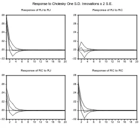
The next step is to do the impulse response analysis. Considering the model error, calculation error and model stability, Monte Carlo method is used to calculate the dynamic response of the corresponding futures return series on the disturbance of endogenous variables (Liu Bin, 2001)[15], and the number of repetitions is 10,000 times when the impulse response is calculated. In picture 6, the solid line is the mean of the impulse response simulated by Monte Carlo, and the dotted lines mean the solid line plus / minus on the two standard errors of the impulse response. Test results are shown in Figure 6 and Figure 7. Figure 6 reflects the unit shock, while Figure 7 reflects the cumulative shock.

It can be seen from Figure 6 that Japanese rubber futures yields and Chinese rubber futures yields will all

be paid a positive impact and return to a stable state in the first three terms when Japanese rubber futures yields have been paid a positive impact. When Chinese rubber futures yields have been paid a positive impact, Japanese rubber futures yields have almost not been paid a impact, but Chinese rubber futures yields will be paid a positive impact and return to a stable state in the first two to three terms. Figure 6 also shows that shocks of Chinese rubber futures yields have no effect on Japanese rubber futures yields, but shocks of Japanese rubber futures yields have a certain extent effect on Chinese rubber futures yields. This is the same with the conclusion, gotten by the former Grange causality test, that “there is a one-way causal relationship from Japanese rubber futures prices to Chinese rubber futures prices and Japanese rubber futures prices have an unidirectional guiding role on Chinese rubber futures prices between Japanese rubber futures prices and Chinese rubber futures prices, and vice versa”.

-.02 .00 .02 .04 .06 .08

2 4 6 8 10121416 1820

Response of RJ to RJ

-.02 .00 .02 .04 .06 .08

2 4 6 8 1012 14161820

Response of RJ to RC

-.02 .00 .02 .04 .06 .08

2 4 6 8 10121416 1820

Response of RC to RJ

-.02 .00 .02 .04 .06 .08

2 4 6 8 1012 14161820

Response of RC to RC

Response to Cholesky One S.D. Innovations ± 2 S.E.

Figure 6. Unit impact map of Chinese and Japanese rubber futures yields’ impulse response

-.04 .00 .04 .08 .12

2 4 6 8 101214161820

Accumulated Response of RJ to RJ

-.04 .00 .04 .08 .12

2 4 6 8 10121416 1820

Accumulated Response of RJ to RC

.02 .04 .06 .08 .10

2 4 6 8 101214161820

Accumulated Response of RC to RJ

.02 .04 .06 .08 .10

2 4 6 8 10121416 1820

Accumulated Response of RC to RC

Accumulated Response to Cholesky One S.D. Innovations ± 2 S.E.

Figure 7. Cumulative impact map of Chinese and Japanese rubber futures yields’ impulse response

This is the same with the conclusion, gotten by the former Grange causality test, that “there is a one-way causal relationship from Japanese rubber futures prices to Chinese rubber futures prices and Japanese rubber futures prices have an unidirectional guiding role on Chinese rubber futures prices between Japanese rubber futures prices and Chinese rubber futures prices, and vice versa”.

0 40 80 120

2 4 6 8 101214161820

Percent RJ variance due to RJ

0 40 80 120

2 4 6 8 101214161820

Percent RJ variance due to RC

0 20 40 60 80 100

2 4 6 8 101214161820

Percent RC variance due to RJ

0 20 40 60 80 100

2 4 6 8 101214161820

Percent RC variance due to RC

Variance Decomposition ± 2 S.E.

Figure 8. Variance decomposition maps of Chinese and Japanese rubber futures yields

Although the impulse response function depicts the impact of a disturbance of endogenous variable on other variables in VAR, but variance decomposition makes changes in the endogenous variables broken down into VAR factor impact, and thus variance decomposition provides relative importance of each random innovation influencing the variables in VAR (Eviews help file). Figure 8 shows that, throughout the forecasting period, 99% of the forecasting variance of RJ is due to the disturbance of RJ, and 1% of the forecasting variance of RJ is due to the disturbance of RC, and these show that the forecasting variance of RJ is mainly due to the impact of RJ. Throughout the forecasting period, 31% of the forecasting variance of RC is due to the disturbance of RJ, and the remaining 69% of the forecasting variance of RC is due to the disturbance of RC, and these show that the forecasting variance of RC is mainly due to the impact of RC (Pindyck, Rubinfeld, 1999[16]; Eviews help file). According to Figure 8 we can also found that, throughout the forecast period, the part of the forecasting variance of RJ due to the disturbance of RC is much less than the part of the forecasting variance of RC due to the disturbance of RJ. This is the same with the conclusion, gotten by the former Grange causality test, that “there is a one-way causal relationship from Japanese rubber futures prices to Chinese rubber futures prices and Japanese rubber futures prices have an unidirectional guiding role on Chinese rubber futures prices between Japanese rubber futures prices and Chinese rubber futures prices, and vice versa”.

V. CONCLUSIONS

Based on the classical regression model, time-varying coefficient model, unit root, co-integration, Granger causality test, VAR, impulse response and variance decomposition, the dynamic relationship between prices of natural rubber futures in China and Japan has been researched systematically. Main conclusions are drawn and some suggestions are put forward as follows through empirical researches: Firstly, there is a stable

co-integration relationship between prices of natural rubber futures in China and Japan. Secondly, whatever in terms of actual economic background or in terms of the model fitting results, the time-varying coefficient model is superior to the classical regression model. Thirdly, the influence of price of natural rubber futures in Japan on price of natural rubber futures in China is time-varying. Every 1% change of Japanese rubber futures prices will lead to 0.4% to 0.6% change of Chinese rubber futures prices. In the long run, the impact of natural rubber futures in Japan on natural rubber futures in China has been gradually increased. Fourth, the influence of price of natural rubber futures in Japan on price in China is greater than the influence of price of natural rubber futures in China on price in Japan, and Japanese rubber futures prices are the granger cause of Chinese rubber futures price, and vice versa. Fifth, with the deepening of China's opening up and the gradual accession to the world after joining the World Trade Organization, the relationship between Chinese natural rubber futures prices and foreign prices are becoming closer, and this also further requires relevant managers and investors in China to have an international outlook, pay close attention to the international price fluctuations of the relative futures, and at advance do well the prevention and response measures to avoid the negative impact of the foreign futures price volatility on our country too much.

ACKNOWLEDGMENT

This work was supported in part by a grant from the National Social Science Fund in China (No. 11CJY080).

REFERENCES

[1] Shanghai Futures Exchange, Trading Manual for contracts of Natural rubber futures, 2008 Edition.

[2] Feature Article, “Analysis on the main factors which

influence the price volatility of China rubber futures,” [J].China rubber, vol. 20(7), pp. 26 -27, 2004.

[3] RENHAI HUA, BAIZHU CHEN, “International Linkages

of the Chinese Futures Markets,” [J]. China Economic Quarterly, vol. 3(3), pp.727-742, 2004.

[4] JIN Tao, Miao Baiqi, HUI Jun, “Investigating the Casual Relationship of the Future Copper Price between LME and SHFE under the Interaction,” [J].OPERATIONS RESEARCH AND MANAGEMENT SCIENCE, vol. 14(6), pp.88-92, 2005.

[5] Zhao Liang, Liu Liya, “Research on the relationship

between copper futures markets at home and abroad,” [J]. TONG JI YU JUE CE, vol. 10, pp.116-118, 2006.

[6] LIU Qing-fu, ZHANG Jin-qing, HUA Ren-hai,

“Information Transmission between LME and SHFE in Copper Futures Markets,” [J]. Journal of Industrial Engineering, vol. 122(12), pp.155-159, 2008.

[7] E. SCHLICHT, “Variance Estimation in a Random

Coefficients Model,”[C].Paper presented at the Econometric Society European Meeting, Munich 1989, http://www.lrz.de/~ekkehart.

[8] Gao Tiemei. Econometric analysis and

[9] Yi huiwen, “Discussion on How to Do Granger Causality Test,” [J]. Journal of the Postgraduate of Zhongnan University of Economics and Law, vol.5, pp.34-36, 2006.

[10]C.W.J. Granger, “Investigating Causal Relations by

Econometric Models and Cross-spectral Methods,” [J]. Econometrica, Vol. 37, No. 3, pp. 424-438, 1969.

[11]ZOU Ping. Financial Econometrics [M]. Shanghai:

Shanghai University of Finance & economics Press, pp.150-183, 2005.

[12]C.A. Sims, “Macroeconomics and reality,” [J].

Econometrica, Vol.48, No.1,pp. 1-48,1980.

[13]SHEN Yue, LIU Hongyu, “Relationship between real

estate development investment and GDP in China,” JT singhua Univ (Sci & Tech), vol. 44 (9), pp.1205-1208, 2004.

[14]Lutkepohl, Helmut. Introduction to Multiple Time Series Analysis. New York: Springer Verlag, 1991.

[15]Liu Bin, “Identification of the impact of monetary policy and empirical analysis on the effectiveness of China's monetary policy,” [J].Journal of Financial Research, vol.7, pp.1-9, 2001.

[16]R.S. Pindyck, D.L. Rubinfeld, Econometric Models and Economic Forecasts[M].Translated by Qian Xiaojun and etc., Beijing: China Machine Press, pp.273-277, 1999.