www.scienceworldjournal.org ISSN 1597-6343
Computations of Scattering Cross Sections for He, Ne, Ar, Kr,
Xe and Rn
*ABDU, S. G.1
1Department of Physics, Kaduna State University, Kaduna-Nigeria
ABSTRACT
Calculated Total Cross-Sections (TCS) of elastic electron-atom
scattering for He, Ne, Ar, Kr, Xe and Rn are presented. The
computed TCS were calculated using the partial wave, Eikonal,
Born, and the optical theorem approximation methods with the
Lenz-Jensen potential, at electron incident energies between
1to1000 eV. Results obtained using the partial wave, Eikonal and
optical theorem approximation methods are in good agreement
with experimental TCS data of Van den Biesen et al (1982).
Keywords: Total Cross-Sections, elastic scattering, noble gases,
partial wave, Eikonal, optical theorem, Born approximation.
INTRODUCTION
In scattering theory, the Total Cross-Section (TCS) is a measure of
the probability that an interaction occurs; the larger the cross
section, the greater the probability that an interaction will take
place when a particle is incident on a target (Anchaver, 2003).
Elastic electron-atom scattering takes place if the final state of an
atom after the interaction coincides with the initial one (Winitzki,
2004). Total and differential cross-sections for such a process can
be calculated in various approximations — Born (Merzbacher,
1970)), Eikonal (Innanen, 2010; Shajesh, 2010), optical theorem
(Lokajicek & Kundrat, 2009; Ronniger, 2006), partial wave method
(Cox & Bonham, 1967), etc. In this work, the total cross-sections of
the noble gases He, Ne, Ar, Kr, Xe and Rn (Halka & Nordstrom,
2010; Ramazanov et al, 2007) were computed using the four
approximation methods listed above.
MATERIALS AND METHODS
We used the FORTRAN code program developed by Koonin &
Meredith (1989) which takes the relativistic differential
cross-section as a sum of squared modules of the real and imaginary
scattering amplitudes. The amplitudes can be calculated through
the phase shifts of spherical waves, which are obtained by
integration of equations for radial wave functions. In these
computations the analytical approximation for the atomic
electrostatic potential given by Lenz and Jensen, called the
Lenz-Jensen
potential (Blister & Hautala, 1978), based on the Thomas-Fermi
model, is used.
Scattering Theory
For particles of mass m and energy
=ℏ > 0 1.0
scattering from a central potential, V(r) is described by a wave
function, ψ(r) that satisfies the Schrodinger Wave Equation (SWE)
−ℏ ∇ + = 2.0
with the boundary condition at large distance
→∞→ + ( ) 3.0
Equation (3.0) holds for a beam of electrons incident along z-axis,
and the scattering angle, is the angle between r and ̂ while is
the complex scattering amplitude, which is the basic function we
seek to determine. The differential cross-section is given by:
Ω= | ( )| 4.0
The total cross-section is
=∫ Ω σ
Ω= 2π∫ dθsinθ|f(θ)| π
5.0
is a function of both and (Koonin & Meredith, 1989).
Approximation Methods
Approximations play a very important role in our understanding of processes that cannot be solved exactly. The calculation of scattering cross sections is one of the most important uses of
Ful
l Le
ngt
h
R
es
ea
rc
h
ISSN 1597-6343
Fermi’s Golden Rule (Wacker, 2011). Fermi’s rule involves only one matrix element of the interaction which makes it a first order approximation to the exact result. This approximation suggests an approximation to the complex scattering amplitude.
The Born approximation involves an approximation to the complex
scattering amplitude (Merzbacher, 1970). It has been extensively
used to study low energy as well as high energy scattering
processes. The Eikonal approximation is a technique for
estimating the high energy behaviour of a forward scattering
amplitude (Innanen, 2010). It was originally developed for potential
scattering in quantum mechanics, where one approximates the
classical trajectory corresponding to forward scattering by a
straight line and uses a WKB approximation for the wavefunction
(Sakuri, 1985). The optical theorem relates the forward scattering
amplitude to the cross section (Lokajicek & Kundrat, 2009).
Partial Wave Method
The method of partial wave expansion is a special trick to simplify
the calculation of the scattering amplitude, (Newton, 1982). The
standard partial wave decomposition of the scattering wave
function is
( ) =∑∞ (2 + 1) ( ) ( ) 6.0
When equation (2.6) is substituted into the SWE (2.0) the radial
wave functions, are found to satisfy the radial differential
equations:
−ℏ + ( ) + ( )ℏ − ( ) = 0 7.0
This is the same equation as that satisfied by a bound state wave
function but the boundary conditions are different. In particular,
vanishes at the origin, but it has the large-r asymptotic behaviour
→ [ ( )− ( )] 8.0
Where and are the regular and irregular spherical Bessel
functions of order .
The scattering amplitude is related to the phase shifts by [9]:
( ) = ∑∞ (2 + 1) ( ) 9.0
From equations (5.0) and (9.0) the total cross-section is given by
= ∑∞ (2 + 1) 10.0
Although the sums in equations (9.0) and (10.0) extend over all ,
they are in practice limited to only a finite number of partial waves.
This is because for large , the repulsive centrifugal potential in
equation (7.0) is effective in keeping the particle outside the range
of the potential and so the phase shift is very small.
If the potential is negligible beyond a radius , an estimate of
the highest partial wave that is important is had by setting the
turning point at this radius:
( )ℏ
= 11.0
⇒ ≈ 12.0
This estimate is usually slightly low since the penetration of the
centrifugal barrier leads to non-vanishing phase shifts in partial
waves somewhat higher than this (Koonin & Meredith, 1989).
The Phase shifts
To find the phase shift in a given partial wave, we must solve the
radial equation (7.0). The equation is linear, so that the boundary
condition at large
can be satisfied simply by appropriately normalizing the solution.
If we put ( = 0) = 0 and take the value at the next lattice
point, ( =ℎ), to be any convenient small number we then use
"≈ 13.0
for "(ℎ), along with the known values (0), (ℎ), and (ℎ)
to find (2ℎ).
Now we can integrate outward in to a radius ( )> . Here,
vanishes and must be a linear combination of the free
solutions, ( ) and ( ):
( )
= ( ) ( ) − ( ) 14.0
Although the constant, above, depends on the value chosen for
( =ℎ), it is largely irrelevant for our purposes; however, it
must be kept small enough so that overflows are avoided. Now
( )
= ( ) ( ) − ( ) 15.0
Equations (14.0) and (15.0) can then be solved for to obtain
=
( ) ( )
( ) ( ); =
( ) ( )
( ) ( ) 16.0
where ( )= ( ( ) etc. Equation (16.0) determines only
within a multiple of but this does not affect the physical
observables [see equations (9.0) and (10.0)]. The correct multiple
of ’s at a given energy can be determined by comparing the
number of nodes in and in the free solution, which occur
for < . The phase shift in each partial wave vanishes at
high energies and approaches at zero energy, where is
the number of bound states in the potential in the ’th partial wave
(Koonin & Meredith, 1989).
The Lenz-Jensen Potential
One practical application of the theory discussed above is the
calculation of the scattering of electrons from neutral atoms. In
general this is a complicated multi-channel scattering problem
since there can be reactions leading to final states in which the
atom is excited. However, as the reaction probabilities are small in
comparison to elastic scattering, for many purposes the problem
can be modeled by the scattering of an electron from a central
potential (Koonin & Meredith, 1989). This potential represents the
combined influence of the attraction of the central nuclear charge
(Z) and the screening of this attraction by the Z atomic electrons.
For a neutral target atom, the potential vanishes at large distances
faster than . A very accurate approximation to this potential
can be had by solving for the self-consistent Hartree-Fock potential
of the neutral atom. However, a much simpler estimate can be
obtained using an approximation to the Thomas-Fermi model of
the atom given by Lenz and Jensen (Blister & Hautala, 1978)
=− (1 + + + + ); 17.0
with
= 14.409; = 0.3344; = 0.0485; = 2.647 × 10 ;
18.0
and
= 4.5397 19.0
This potential is singular at the origin. If the potential is regularized
by taking it to be a constant within some small radius (say
the radius of the atom’s 1s shell), then the calculated cross-section
will be unaffected except at momentum transfers large enough so
that ≫1.
The incident particle is assumed to have the mass of the electron,
and, as is appropriate for atomic systems, all lengths are
measured in angstrom (Å)
and all energies in electronvolt (eV). The potential is assumed to
vanish beyond 2Å. Furthermore, the singularity in the potential
is cutoff inside the radius of the 1s shell of the target atom.
Research Methodology
A FORTRAN program developed by Koonin & Meredith (1989)
was the main program used for all the computations. The program
is made up of four categories of files: common utility programs,
physics source code, data files and include files. The physics
source code is the main source code which contains the routine for
the actual computations. The data files contain data to be read into
the main program at run-time and have the extension .DAT. The
first thing done was the successful installation of the FORTRAN
codes in the computer. This requires familiarity with the computer’s
operating system, the FORTRAN compiler, linker, editor, and the
graphics package to be used in plotting. The program runs
interactively. It begins with a title page describing the physical
problem to be investigated and the output that will be produced.
Next, the menu is displayed, giving the choice of entering
parameter values, examining parameter values, running the
program, or terminating the program. When the calculation is
finished, all values are zeroed (except default parameters), and the
main menu is re-displayed, giving us the opportunity to redo the
calculation with a new set of parameters or to end execution. Data
generated from the program were saved in files which were later
imported into the graphics software Origin 5.0 for plotting.
RESULTS
Results were generated for several electron incident energies as
presented in the tables below:
ISSN 1597-6343
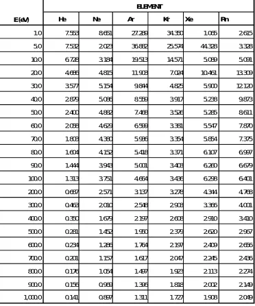
From table 1 below, using the partial wave method, we observed
that the TCS for He decrease with increasing electron incident
energies from 1 to 1,000 eV. The TCS for Ne, Ar, Xe and Rn
exhibited a number of minima and maxima between 1 to 100 eV,
but decrease with increasing incident energies between 100 to
1,000 eV. Also, the TCS increase with increasing atomic number
for all elements considered. The differences in TCS for He, in the
energy range of about 70 to 1,000 eV, are substantially higher than
differences in TCS for other noble gases. This might have resulted
from the fact that He has an “S” valance shell only while all the
others have “P” valence shells.
Table 1: Computed Total Cross-Sections for Elastic Electron- Atom Scattering for He, Ne, Ar, Kr, Xe and Rn using the Partial Wave Method with the
Lenz-Jensen Potential.
He Ne Ar Kr Xe Rn
1.0
7.553 8.651 27.289 34.350 1.065 2.615
5.0
7.532 2.023 36.882 25.574 44.328 3.328
10.0
6.728 3.184 19.513 14.571 5.089 5.091
20.0
4.686 4.815 11.903 7.024 10.461 13.309
30.0
3.577 5.154 9.844 4.825 5.900 12.120
40.0
2.879 5.086 8.559 3.917 5.238 9.873
50.0
2.400 4.882 7.468 3.526 5.285 8.611
60.0
2.058 4.629 6.599 3.381 5.547 7.870
70.0
1.803 4.380 5.936 3.354 5.854 7.375
80.0
1.604 4.152 5.418 3.371 6.107 6.997
90.0
1.444 3.943 5.001 3.403 6.260 6.679
100.0
1.313 3.751 4.664 3.436 6.298 6.401
200.0
0.687 2.571 3.137 3.278 4.344 4.768
300.0
0.463 2.010 2.548 2.903 3.366 4.001
400.0
0.350 1.679 2.197 2.608 2.910 3.410
500.0
0.281 1.452 1.950 2.379 2.620 2.967
600.0
0.234 1.286 1.764 2.197 2.409 2.656
700.0
0.201 1.157 1.617 2.047 2.245 2.436
800.0
0.176 1.054 1.497 1.923 2.113 2.274
900.0
0.156 0.969 1.396 1.818 2.002 2.149
1,000.0
0.141 0.897 1.311 1.727 1.908 2.049 E (eV)
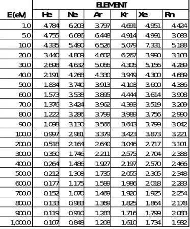
From table 2 , using the Eikonal method, the TCS for He also decrease with increasing electron incident energies from 1 to 1,000 eV. The TCS for Ne, Ar, kr, Xe and Rn exhibited a number of minima and maxima between 1 to 30 eV, but decrease with increasing incident energies between 30 to 1,000 eV. Also, the
TCS increase with increasing atomic number for all elements considered. The differences in TCS for He, in the energy range of about 50 to 1,000 eV, are substantially higher than differences in TCS for other noble gases.
Table 2: Computed Total Cross-Sections for Elastic Electron- Atom Scattering for He, Ne, Ar, Kr, Xe and Rn using the Eikonal Approximation Method with
the Lenz-Jensen Potential..
He
Ne
Ar
Kr
Xe
Rn
1.0
4.784
6.203
3.797
4.691
4.951
4.424
5.0
4.755
6.686
6.448
4.914
4.991
3.083
10.0
4.335
5.490
6.526
5.079
7.331
5.188
20.0
3.440
4.809
4.602
6.267
3.990
3.103
30.0
2.698
4.632
5.066
4.305
5.156
4.289
40.0
2.191
4.268
4.330
3.949
4.300
4.689
50.0
1.834
3.740
3.913
4.103
3.600
4.386
60.0
1.573
3.538
3.895
4.444
3.614
3.908
70.0
1.376
3.424
3.962
4.393
3.519
3.269
80.0
1.222
3.286
3.799
3.989
3.756
2.990
90.0
1.098
3.130
3.566
3.643
3.799
3.042
100.0
0.997
2.981
3.379
3.423
3.873
3.221
200.0
0.518
2.164
2.640
3.046
2.717
3.101
300.0
0.350
1.746
2.211
2.575
2.704
2.388
400.0
0.264
1.486
1.927
2.197
2.570
2.466
500.0
0.212
1.308
1.735
2.055
2.305
2.348
600.0
0.177
1.175
1.589
1.986
2.018
2.283
700.0
0.152
1.070
1.469
1.920
1.925
2.254
800.0
0.133
0.983
1.369
1.825
1.864
2.178
900.0
0.119
0.910
1.283
1.716
1.799
2.083
1,000.0
0.107
0.848
1.208
1.610
1.734
1.932
E (eV)
ELEMENT
ISSN 1597-6343
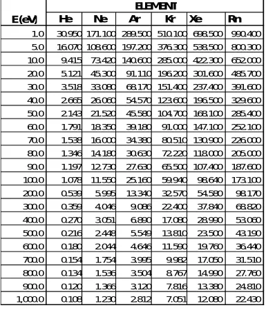
From table 3, using the Born method, the calculated TCS are significantly higher than the TCS obtained using the three other approximation methods. This is as a result of the fact that the Born approximation is only valid at high electron incident energies. As
previously observed, the calculated TCS decrease with increasing incident energies but no minima and maxima were observed for all the elements considered.
Table 3: Computed Total Cross-Sections for Elastic Electron- Atom Scattering for He, Ne, Ar, Kr, Xe and Rn using the Born Approximation Method with the
Lenz-Jensen Potential..
He
Ne
Ar
Kr
Xe
Rn
1.0
30.950 171.100 289.500 510.100 698.500
990.400
5.0
16.070 108.600 197.200 376.300 538.500
800.300
10.0
9.415
73.420 140.600 285.000 422.300
652.000
20.0
5.121
45.300
91.110 196.200 301.600
485.700
30.0
3.518
33.080
68.170 151.400 237.400
391.600
40.0
2.665
26.060
54.570 123.600 196.500
329.600
50.0
2.143
21.520
45.580 104.700 168.100
285.400
60.0
1.791
18.350
39.180
91.000 147.100
252.100
70.0
1.538
16.000
34.380
80.510 130.900
226.000
80.0
1.346
14.180
30.630
72.220 118.000
205.000
90.0
1.197
12.730
27.630
65.500 107.400
187.600
100.0
1.078
11.550
25.160
59.940
98.640
173.100
200.0
0.539
5.995
13.340
32.570
54.580
98.170
300.0
0.359
4.046
9.086
22.400
37.840
68.820
400.0
0.270
3.051
6.890
17.080
28.990
53.060
500.0
0.216
2.448
5.549
13.810
23.500
43.190
600.0
0.180
2.044
4.646
11.590
19.760
36.440
700.0
0.154
1.754
3.995
9.982
17.050
31.510
800.0
0.134
1.536
3.504
8.767
14.990
27.760
900.0
0.120
1.366
3.120
7.816
13.380
24.810
1,000.0
0.108
1.230
2.812
7.051
12.080
22.430
E (eV)
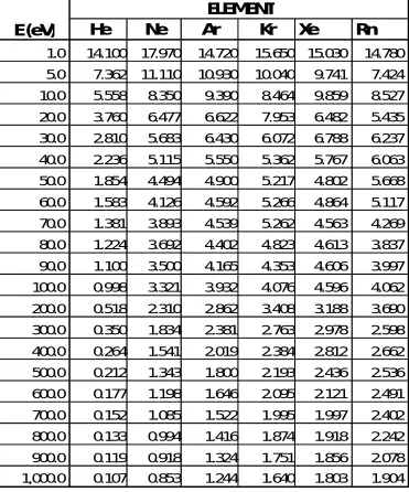
From table 4 and fig. 4, using the optical theorem method, the calculated TCS for Kr, Xe and Rn exhibited a number of minima and maxima in the energy range of 1 to 100 eV. No minima or maxima were observed for He, Ne and Ar. Here also, the calculated TCS decrease with increasing electron incident energies.
The calculated TCS using the partial wave, Eikonal and optical theorem approximation methods are generally in good agreement with the experimental TCS obtained by Van den Biesen et al (1982). However TCS calculated using the Born approximation method are much higher than the experimental values for the energy range considered. This is because the Born approximation is only valid at high electron incident energies.
Table 4: Computed Total Cross-Sections for Elastic Electron- Atom Scattering for He, Ne, Ar, Kr, Xe and Rn using the Optical Theorem with the Lenz-Jensen
Potential.
He
Ne
Ar
Kr
Xe
Rn
1.0
14.100
17.970
14.720
15.650 15.030
14.780
5.0
7.362
11.110
10.930
10.040
9.741
7.424
10.0
5.558
8.350
9.390
8.464
9.859
8.527
20.0
3.760
6.477
6.622
7.953
6.482
5.435
30.0
2.810
5.683
6.430
6.072
6.788
6.237
40.0
2.236
5.115
5.550
5.362
5.767
6.063
50.0
1.854
4.494
4.900
5.217
4.802
5.668
60.0
1.583
4.126
4.592
5.266
4.864
5.117
70.0
1.381
3.893
4.539
5.262
4.563
4.269
80.0
1.224
3.692
4.402
4.823
4.613
3.837
90.0
1.100
3.500
4.165
4.353
4.606
3.997
100.0
0.998
3.321
3.932
4.076
4.596
4.062
200.0
0.518
2.310
2.862
3.408
3.188
3.690
300.0
0.350
1.834
2.381
2.763
2.978
2.598
400.0
0.264
1.541
2.019
2.384
2.812
2.662
500.0
0.212
1.343
1.800
2.193
2.436
2.536
600.0
0.177
1.198
1.646
2.095
2.121
2.491
700.0
0.152
1.085
1.522
1.995
1.997
2.402
800.0
0.133
0.994
1.416
1.874
1.918
2.242
900.0
0.119
0.918
1.324
1.751
1.856
2.078
1,000.0
0.107
0.853
1.244
1.640
1.803
1.904
E (eV)
ELEMENT
ISSN 1597-6343 CONCLUSION
Computed Total Cross-Sections (TCS) of elastic electron-atom scattering for the elements He, Ne, Ar, Kr, Xe and Rn are presented. The TCS were calculated using the partial wave, Eikonal, Born, and the optical theorem approximation methods with the Lenz-Jensen potential, at incident energies of 1to1000 eV. Results obtained using the partial wave, Eikonal and optical theorem methods are in good agreement with the experimental TCS values.
REFERENCE
Anchaver, R.S. (2003), Introduction to Non-relativistic Quantum Mechanics, Identity Books, Kano-Nigeria.
Blister, M. and Hautala, M. (1978), Calculation of the Lenz-Jensen Potential Using the Third Order Approximation, Physics Letters A, 68 (1), pp. 98-100.
Cox, H.L. and Bonham, R.A. (1967), Elastic Electron Scattering Amplitudes for Neutral Atoms Calculated Using the Partial Wave Method at 10, 40, 70 and 100kV for Z=1 to Z=54, J. chem.. Phys., 47, pp. 2599.
Halka, M. and Nordstrom, B. (2010), Halogens and Noble Gases, Facts On File, New York.
Innanen, K.A.(2010), A Scattering Diagram Derivation of the Eikonal Approximation. Available at
www.crewes.org/ForOurSponsors/ConferenceAbstracts/2010/CSE G/Innanen_GC_2010.pdf Accessed on 21/06/2011.
Koonin, S.E. and Meredith, D.C. (1989), Computational Physics (FORTRAN Version), Addison-Wesley, New York.
Lokajicek, M.V. & Kundrat, V. (2009), Optical Theorem and Elastic Nucleon Scattering, arXiv: 0906.396 1v1 [hep-ph].
Merzbacher, E. (1970), Quantum Mechanic, 2nd ed., J. Wiley & Sons Inc., New York.
Newton, R.G. (1982), Scattering Theory of Waves and Particles, 2nd ed., Springer-Verlag, Berlin.
Ramazanov, T.S., Dzhumagulova, K.N., Omarbakiyeva, Y.A. and Ropke, G. (2007), Scattering of Low-Energy Electrons by Noble Gas Atoms in Partially Ionized Plasma, 34th EPS Conference on Plasma Physics, Warsaw, ECA, vol. 31F, pp. 2.093.
Ronniger, M. (2006), The Optical Theorem and Partial Wave Unitarity, Seminars on Theoretical Particle Physics, University of Bonn, held 29/06/2006 (unpublished).
Sakuri, J.J. (1985), Modern Quantum Mechanics, Addison-Wesley, New York.
Shajesh, K.V. (2010), Eikonal Approximation, Available at http://www.nhn.ou.edu/~shajesh/eikonal/sp.pdf Accessed 12/10/ 2010.
Van den Biesen, J.J.H., Herman, R.M. and Van den Meijdenberg, C.J.N. (1982), Experimental Total Collision Cross Sections in the Glory Region for Noble Gas Systems, Physica A, 115 (3), pp. 396-439.
Wacker, A. (2011), Fermi’s Golden Rule. Available at
www.matfys.lth.se/Andreas.Wacker/Scripts/fermiGR.pdf Accessed on 22/06/2011.
Winitzki, S. (2004), Scattering Theory Lecture Notes, Uni-Muenchen. Available at