Optimization of Multiple Gateway Deployment for
Underwater Acoustic Sensor Networks
Jugen Nie1,2, Deshi Li1, and Yanyan Han1
1 School of Electronic Information, Wuhan University 430079 Wuhan, China
2 School of Electronic and Information Engineering, Jinggangshan University 343009 Ji’ an, China
{ niejugen, hanyan4981}@163.com
Abstract. This research aims to develop novel technologies to efficiently integrate wireless communication networks and Underwater Acoustic Sensor Networks (UASNs). Surface gateway deployment is one of the key techniques for connecting two networks with different channels. In this work, we propose an optimization method based on the genetic algorithm for surface gateway deployment, design a novel transmission mechanism—simultaneous transmission, and realize two efficient routing algorithms that achieve minimal delay and payload balance among sensor nodes. We further develop an analytic model to study the delay, energy consumption and packet loss ratio of the network. Our simulation results verify the effectiveness of the model, and demonstrate that the technique of multiple gateway deployment and the mechanism of simultaneous transmission can effectively reduce network delay, energy consumption and packet loss rate. Keywords: Underwater acoustic sensor networks, gateway deployment, transport mechanism.
1.
Introduction
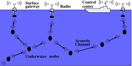
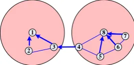
multipath interference, and many other transmission attenuation factors. Therefore it becomes a highly challenging wireless communication channel. The propagation speed of underwater acoustic signal (approximately 1500m/s, with variation due to minor changes of pressure, temperature, and salinity of water) is lower than electromagnetic wave propagation speed by five orders of magnitude; such high propagation delay will not only limit the interactive application, but also prolong the response time of communication. Compared to its single gateway counterpart, data in a underwater sensor network with multiple gateways (Fig. 1) do not have to be transmitted via a long path to a fixed surface gateway, but via a path selected in light of optimized network performance (such as minimal delay, minimal energy consumption and least packet loss rate) to one of the available gateways [5]. Depends on the service requirement, the surface gateways can adopt various wireless communication channels such as Cellular network, Zigbee and so on. Note that the data propagation delay from surface gateways to the base station is much shorter than that in underwater acoustic network. The bandwidth of wireless channel can vary from tens of million to hundreds of million bits per second; in a sharp contrast, the data rate of underwater acoustic channel is only between several hundred bits and ten kilobits per second. Moreover, the packet loss rate of surface gateways is much smaller than that of underwater acoustic network. Also compared to radio communication, acoustic communication needs much more energy [6]. The surface gateways can obtain power supply from solar panels or by changing battery periodically. Due to the aforementioned factors, an underwater sensor node can select a path to one of these gateways, aiming to minimize the delay, energy consumption or packet loss rate from it to the gateway. Therefore, how to design an efficient routing algorithm according to different optimization goals, how to select the number and the position of surface gateways are the key research issues of the UASNs with multiple gateways.
Radio
Acoustic Channel Surface
gateway
Control center
Underwater nodes
Fig. 1. Structure of Multiple Gateway UASNs
Networks
routing of data packets from underwater sensor nodes to surface gateways under various objects was not studied.
In this work, we assume that the coordinates of underwater sensor nodes
are known.We show how routing is discovered under various objectives such
as minimal delay and payload balance, and design a novel transmission mechanism—simultaneous transmission. We further develop an analytic model to study the delay, energy consumption and packet loss ratio of the network. As a result, we verify the effectiveness of the model.
The rest of the paper is organized as follows. Sec. 2 illustrates the related works of multiple gateway deployment. Sec. 3 presents the model for optimization of multiple gateway deployment. Sec. 4 proposes a new mechanism of simultaneous transmissions. Sec.5 describes the process of route discovery. Sec.6 describes gateway deployment based on GA. Sec. 7 discusses simulation results. Finally, Sec. 8 concludes the paper.
2.
Related Works
Deployment of multiple gateway in wireless networks can be divided into two categories: one is terrestrial wireless networks, and the other is multiple surface gateway deployment in UASNs.
Most multiple gateway deployment research in terrestrial wireless networks is mainly on the gateway site selection in wireless mesh networks (WMNs). Literature [7] proposed a new routing algorithm called two concurrent path routing (2CPR) for wireless mesh networks with multiple gateways. Literature [8] proposed a gateway selection scheme that considers multiple end-to-end QoS parameters. Literature [9] presented a multiple gateway selection algorithm for WMNs called Weighted Clustering Algorithm (WCA), which is an optimization mechanism based on the Quality of Service (QoS), and used a heuristic algorithm to improve the performance of WCA. The core of WCA is determining the number and location of gateways. However, WCA assumes that nodes locations are known, so that some nodes can be selected as gateways for cluster planning. Aforementioned research focuses on the selection of gateway. For the number of gateways has been pre-determined, the algorithm aimed at selecting the gateway with balanced payload in the network, but did not refer to the gateway position and the effect of gateway number. Literature [10] combined graph partition and spanning tree algorithm, but how to get good computational efficiency of this algorithm is one problem.
gateways should be focused on the propagation delay from underwater sensor nodes to gateways, energy consumption of underwater nodes and packet loss rate.
For multiple gateway deployment in UASNs, Literature [11] gave a triangular deployment method of 2-dimensional network, and it was aimed at target area coverage with minimal sensors. Literature [12] studied the coverage and routing in 3-dimensional networks. Neither of the two studies involved network structure with multiple sinks nodes (or gateways). Literature [13] used multiple sink nodes to improve the performance of UASNs, but they did not analyze the influence of network delay and energy consumption with multiple gateways. Literature [14] proposed the architecture of surface gateway that has several wireless communication channels and communication protocols. However, they didn’t study the effect of the gateway number and positioning. Literature [6][15] focused on how many gateways should be used, and then derived the positions of multiple gateway from the fixed grid on the surface. The queuing delay due to MAC protocol is not considered, the deployment of surface gateways is not resolved with heavy network payload, and the preliminary simulation results were obtained only for one layer (which is 100 meters below the surface). For most of the applications, underwater sensor network would be a 3-dimensional network, because of limited available bandwidth and low signal propagation speed of underwater acoustic channel, data packet collisions, avoidance and reservation in MAC layer protocol will inevitably bring about queuing delay. At the same time, different transport mechanisms will also affect data transmission delay and energy consumption in network, these problems should be considered for 3-dimension UASNs.
To solve the above issues, this paper proposes a new method of surface gateway deployment. Its main idea is to take the fixed underwater nodes as source nodes and the movable surface gateways as destination nodes. We design a novel transmission mechanism—simultaneous transmissions by nodes which are separated by three hops and realize two efficient routing algorithms that achieve minimal delay and payload balance among sensor nodes.
With the delay, energy consumption and packet loss ratio of network as the optimization objectives, we can obtain the optimal positions of surface gateways and a routing that can optimize network performances.
3.
Optimization Model
Networks 3.1. Definitions
3.1.1 Nodes
Here let V denote all the underwater sensor nodes, G be all the surface gateways, V′ denote all nodes, that is to say V′=V∪G. I(v) denotes all nodes in the communication range of node v, i.e., I(v)={w:wV′, v≠w, d(v,w)≤R}, where d(v,w) is the distance between v and w, and R is the communication range of sensor nodes.
3.1.2 Edges
Let E be all the edges e=(v,w), vV,wI(v), and e(v,u)={e(v,u):(v,u) vE,
uI(v)} denote the direction from node v to node u. For any surface gateway
node, because the data relaying rate of surface gateways is much higher than underwater nodes, so it doesn’t need to consider the relay delay in UASNs. Therefore we can mainly focus on the receiving data for gateways.
3.1.3 Gateway Position
G(X,Y) denotes all surface gateway positions; Gi (xi, yi) is the position of the ith gateway.
3.1.4 Queuing Delay of MAC
Tmac is the delay caused by MAC layer, which is associated with the
connectivity degree of a node. For simplicity, let tm be the queuing delay of
one unit. The queuing delay with only one neighbor is set to Tmac=0, then the
queuing delay caused by two one-hop neighbors is Tmac= tm, three neighbor
links lead to the queuing delay Tmac= 2tm; and so on. For a node with n
neighbors, its queuing delay is approximated as (n-1) tm.
3.2. Constraints
In current UASNs, half-duplex communication mode is often adopted. Therefore we set a simple conflict model: when a node is receiving data, it could not send data simultaneously.
3.3. Optimization Variables
We set two optimization variables: the number of surface gateways N and the
position of surface gateways G (X, Y). Because gateways are located on the
is to optimize N and Gi (xi, yi) according to the objective functions introduced below.
3.4. Optimization Function
3.4.1 Minimum Delay
The goal is to minimize the total delay of all packets that reach the surface gateway. Packet delay is the sum of all delays generated from every hop along the path from the transmitter to the receiving gateway. Combining queuing delays of the relay-nodes (resulted from the MAC layer or routing layer), delay of each hop composites of transmission delay, queuing delay
and propagation delay, the delay t of data on edge e can be written as
( )
( ) ( ) ( ) ( ) e
mac s p m
p
L d e
t e t e t e t e n t
C v
(1)
Here, tmac(e) represents queuing delay, ts(e) represents transmission delay and tp(e) denotes propagation delay, n is the connectivity degree of a receiving node (i.e., the number of neighbor nodes in the spanning tree), tm is the connectivity degree associated with unit queuing delays, Le is a total length of transmitted data packet in unit of bit, including all data generated by the sending node and data to be relayed by the next hop, C is the channel capacity in unit of bit/sec, d(e) is the edge length, vp is the underwater acoustic propagation speed.
Therefore, the objective function of minimum total delay is
( )
t e Minimize
E e r
(2)
Where Er stands for all edges of the route spanning tree from the underwater
nodes to gateway. Obviously, eEr. 3.4.2 Minimum Energy Consumption
The goal is to achieve the minimum energy consumption when all the packets have been transmitted to the surface gateway. If a node sends data
Lv, the energy it consumes can be written as
( )v Ps( )v ts Pr( )v tr s( )v P vr( ) Lv
C P
(3)
Here, Ps(v) is the transmitting power of node v, Pr(v) is the receiving power of node v. ts and tr denote transmission time and reception time respectively. C is the channel capacity in unit of bit/sec.
Networks
( )
Minimize v
v V
(4)
3.4.3 Minimum Packets Loss Rate
Packet loss may be resulted from the physical layer, MAC layer, network congestion and other factors. For example, when the data generation period of a node is less than the minimum period required for network transmission, the data must be stored in the memory of a relay-node, and when the memory is full, the data will overflow possibly leading to packet loss. Here considering packet loss generated when traffic constraint is not satisfied, the optimization objective is to minimize packet loss rate of all packets reaching the surface gateway. The packet loss rate of each node can be expressed as:
( )v fv C C
(5)
Here fv represents the flow of the node. When fv>C, it indicates that there
is packet loss; when fv≤C, the above formula is zero or negative, and thus there is no packet loss.
The packet loss rate of the whole network is (Lv C)
v V m C
, (6)
where m is the total number of underwater nodes.
The corresponding objective function is:
( )
Minimiz
(7)
4.
Data Transmission Mechanism
The state-of-the-art UASNs protocols fall in to two categories: one is based on the mechanism of competition, and the other is based on the mechanism of time sequence [16]. In order to reduce the delay and energy consumption caused by packet collision and retransmission, we adopt the TDMA scheme of MAC protocol in this research. As the positions of underwater sensor nodes are known, the positions of surface gateways and the route from underwater
nodes to gateways can be obtained according to the optimization objective
functions (i.e., minimal delay, minimal energy consumption or least packet loss rate). We make use of the initialization method in literature [17], allocate time slots to nodes, and at the same time, send the information of synchronization and routing to underwater nodes by surface gateways. Then the data of underwater nodes will be transmitted according to the routes and time slots periodically.
previous hop until the surface gateway is reached), and the transmission can be based on the Shortest path transport mechanism, Accumulated transmission hop by hop, or Mechanism of simultaneous transmission every three hops.
4.1. Shortest Path Transport Mechanism
With the shortest path transport mechanism, data generated by each node will be transferred to the surface gateway nodes via the shortest path.
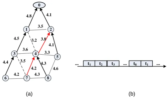
As shown in Figure 2(a), each node chooses the shortest gateway from it as the destination, uses the shortest path to reach the gateway. The total delay is the sum of delays of all data packets reaching gateway. The dotted lines indicate the connections, and the solid lines represent the actual transmission paths (numbers beside lines denote delay). Figure 2(b) represents the time sequence. By this method, the time slot of every node could be selected arbitrarily.
When UASNs is small, low delay could be achieved with the shortest path transport mechanism, because the primary delay here is the transmission delay.
2 1
3 4
5
6 7 8
4.1 4.8
4.5 3.2
3.5 3.6
4.4
3.5
4.2
3.8
4.2 3.3
4.3
4.3 4.1
4.6 0
... t8 t3
t1 t2 t1 ... ...
(a) (b)
Fig. 2. Shortest Path Transport Mechanism
4.2. Accumulated Transmission Hop-by-Hop
Networks
previous hops. The last hop node initiates data transmitting, and accumulates the data ahead hop by hop. The total delay constitutes of transmission delay and propagation delay on the edge with minimum distance as routing edge. In comparison with Figure 2(a), it is obvious that the resulting routing paths are different, as node 4 and node 7 in the Figure 3(a) (numbers beside lines denotes delay). Nodes 7 and 4 select nodes 1 and 3 as the next hop node, respectively, which have smaller delay among the previous hop nodes. Figure 3(b) is the corresponding time sequence. Compared with Figure 2(b), its time sequence must firstly be τ3, τ2 and τ1. Nodes with the same hop
number can arbitrarily select their time slots.
Compared with the shortest path transmission mechanism, this approach yields a smaller total delay when there are more hops, because it reduces repeated transmission delay.
2 1
3 4
5
6 7 8
4.1 4.8
4.5 3.2
3.5 3.6
3.5
4.2
3.8
4.2 3.3
4.3
4.3 4.1
4.6 0
t6 ...
τ3 τ2 τ1
t7 t8 t3 t1 t2 t6
τ’3
...
k i i k
t
denotes all the number of the kth skip
ik
(a) (b) Fig. 3. Accumulated Transmission Hop-by-hop
4.3. Simultaneous Transmission every Three Hops
1 3 9 12 5 2 4 8 11 7 6 10 15 14 13 16 L15 L16
L4 L5 L6
(b) state of simultaneous transmission every two hops (a) initial spanning tree
1 3 9 12 5 2 4 8 11 7 6 10 15 14 13 16
Fig. 4. Simultaneous Transmissions every Three Hops
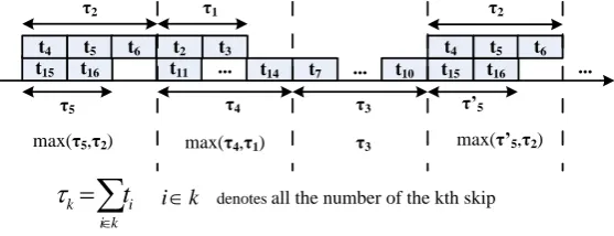
Figure 5 is the corresponding time sequence of data transmission. Similar to figure 3(b), the last hop and its previous three hops firstly send data simultaneously, take the largest delay in the group of nodes as the transmission delay of this group, then the second last hop and its previous three hops send data simultaneously to gateway, and a period of data collection is completed. Figure 5 also shows, when nodes of the third last hop (τ’5 in the figure) send data in the first period, node of the last hop can send
data in the second period (τ5 in the figure). Obviously, this transmission
scheme can efficiently reduce the delay of the whole network.
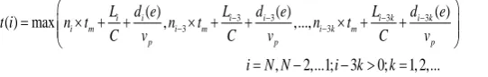
With simultaneous transmission every three hops, the minimum delay in the corresponding optimization model must use formulas 8 and 9 instead of formulas 1 and 2; the delay consumed in the transmission of every hop is:
3 3 3 3
3 3
( ) ( ) ( )
( ) max , ,...,
, 2,...1; 3 0; 1, 2,...
i i i i i k i k
i m i m i k m
p p p
L d e L d e L d e
t i n t n t n t
C v C v C v
i N N i k k
(8)
where ni×tm is the waiting delay of all nodes of the ith hops, Li/B is all the transmission delay of the ith hop, di/vp is all propagation delay of the ith hop,
N is the maximum number of hops.
The total delay of all the packets can be expressed as:
1
[ ( )] ( )
N
i
Minimize t e t i
Networks
t15
τ5 τ4 τ3
t16
t4 t5 t6
t11 t14
τ’5
t2 t3
... t7 ... t10 t15 t16 ...
t4 t5 t6
τ2 τ1 τ2
max(τ5,τ2) max(τ4,τ1) τ3
denotes all the number of the kth skip
k i
i k
t
ikmax(τ’5,τ2)
Fig. 5. Time sequence of Data transmission
5.
Route Discovery
The underwater nodes, surface gateways and the links between them can be abstracted as a connected graph. To obtain the available routes, the underwater nodes can be viewed as source nodes and surface nodes can be viewed as destination nodes. So the network routes Forms the structure of the minimum spanning trees derived from different objective functions.
5.1. Minimum Delay Spanning Tree
There is an exceptional case we must consider as shown in Figure 7.
Assuming nodes 2 and 3 generate data of length L, acoustic speed is vp, the
distance between nodes is d, channel capacity is C, so the time when data
arrives at relay-node 1 before adjusting the spanning tree is T=
2tm+(d2,1+d3,1)/vp+2L/C, and after adjusting the spanning tree, the time T′=2tm+(d2,1+d3,2)/vp+3L/C, so the delay is changed by ΔT=L/C-(d3,1-d3,2)/vp.
When ΔT is negative, it denotes the delay is decreased, so the adjustment is
effective.
Finding the edges between vertexes and endpoints
Save the shortest edge, remove other edges
Removing all connected endpoint to vertex set
Endpoint Set=Ø
Yes
No
Finding the leaf points and vertex set connected them
Finding the shorted edge of every leaf between leaves and
vertexes
Substitute the minimum edge with edges generated ahead
Total delay decrease
End
No Yes
No No
Yes
Spanning tree adjusted?
Yes
leaf set=vertex set Comput ΔT
Vertex Set=Gateways Endpoint Set=underwater nodes
one endpoint connects one vertexes
Fig. 6. Flow Chart of Constructing Minimal Delay Spanning Tree
Networks
path, and substitute the minimum edge for connected edges with leaf node in the spanning tree. Judge whether delay is decreased, if so, replace the old edges with new ones in the spanning tree, continue this process until all leaf nodes have been determined, and then remove the leaf nodes and edges connected with them in the spanning tree, find the new leaf in the residual tree. As the judgment mentioned above, the decreased propagation delay and increased transmission delay are (transmission delay is (n +1) * L / C, in which n is the number of nodes whose data should be relayed via this leaf node in the initial spanning tree connected) determined until there is no need for adjustment of spanning tree, at this time, the spanning tree with minimum total delay is obtained. Figure 8 and figure 9 are the minimum delay trees derived by 2-dimensional simulation, and figure 8 is Spanning tree before adjustment while figure 9 is that after adjustment.
3 1
2
3 1
2
T=tmac(2)+ts(2)+tp(2)+tmac(3)+ts(3)+tp(3)
=tm+d2,1/vp+L/C+tm+d3,1/vp+L/C
T′=tmac(2)+ts(2)+tp(2)+tmac(3)+ts(3)+tp(3)
=tm+d2,1/vp+2L/C+tm+d3,2/vp+L/C
ΔT=T′-T=L/C-(d3,1-d3,2)/vp
Fig. 7. The Adjustfment of Total Delay.
Fig. 9. The Adjusted Minimum Delay Spanning Tree of 2-dimensional Diagram
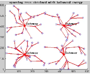
5.2. Minimum Spanning Tree with Balanced Energy
In UASNs, the energy consumption is one of the key issues we concern about, but how to balance all network nodes, and make the network connectivity as long as possible is one of the research emphasis in UASNs area. The energy consumption of a node is related to the data transmission and reception of the nodes. Therefore in order to achieve balanced energy in the network, we can solve the problem in a perspective of the balance between transmitting data and receiving data. The amount of data being sent and received by a node is inversely proportional to the node connectivity degree; energy balance can be realized when network connectivity degree of node is the smallest, and total energy consumption can be minimized when the hop number of every node is the smallest. Therefore, to achieve energy balanced minimum spanning tree, we can first create spanning tree by the minimum hop number.
Networks
the adjustment of this node is completed, and then removes it from the relay-node set. Judge whether the relay-relay-node set is empty, if it is, it denotes that the adjustment of all nodes has completed. Figure 12 is a 2-dimensional minimum spanning tree with balanced energy.
Finding the edges between vertexes and endpoints
Save the shortest edge, remove other edges
Removing all connected endpoint to vertex set
Endpoint Set=Ø
Yes No
Finding all the relay nodes
find the heaviest payload relay node and the
corresponding endpoints set Replace the initial edge with the new edge in
spanning tree Maximum payload
is decreased
No
Yes
No
No Yes
the endnodes set=Ø
Yes
find the shortest egde connected endpoint set with
other nodes Vertex Set=Gateways
Endpoint Set=underwater nodes
One endpoint connects
one vertexes put the point into neighbor relay nodes connected with
the shortest edge
Compute the adjusted maximum payload
End the relay nodes set=Ø
Yes
update maximum payload
Remove the point from relay node set
No
Fig. 10. Flow Chart of Minimum Spanning Tree Obtained with the Objective of Balanced Energy
4 8
5 6
7 1
2 3
Fig. 12. 2-dimensional Spanning Tree Obtained with the Objective of Balanced Energy
6.
Gateway Deployment Based on GA
Genetic algorithm is a global optimized probability searching algorithm, which simulates the evolution process of creature in nature. The population consists of multiple individuals, and it is the computation object, by a repeating iterative process, the individuals will be continuously put on genetic and evaluative operation, and individuals with higher fitness will be transferred to the next generation via the principle of survival of the fittest. So the ultimate result is that individuals with the highest fitness. Because it is a heuristic search based on population, it will find multiple solutions satisfying different preferences in one optimization if it is used in the problem of multiple objectives optimization, and it can handle the objective functions and constraints of all types. Here, we adopt the genetic algorithm, where genetic individual is set to be x coordinate and y coordinate of surface gateways, and the search scale is set to the surface area that underwater nodes corresponds to.
Networks
parameters (the minimal gateway number making network performance optimal).
7.
Simulation and Analysis
7.1. Simulation Setup
In order to evaluate the performance of multiple gateway optimal deployment, we simulate a UASN as shown in Figure 13. The packet length is set as L= 400 bits. The underwater sound propagation velocity is vp = 1500m/s, transmission power Ps(v)= 1 watt, and reception power Ps(v)= 0.2 watt. Note that although data packet collision, avoidance, reservation, and waiting cause power consumption in the MAC layer, such power is generally far less than the transmission power. Also the network is randomly deployed
in an area of 600m × 600m × 600m, where the largest sound communication
distance of underwater sensor nodes and gateway nodes is R = 150m. All underwater sensor nodes are arranged randomly and network connectivity can be maintained. The surface gateway location selection uses GA, running parameters are: the sample size is 40, individual length is 25, number of generations is 25, crossing probability is 0.7, and mutation probability is 0.028. The minimum value of each objective function is regarded as a target. The MAC layer adopts TDMA.
600m 600m
node Number =100
600m
Fig. 13. The Configured Scene for Our Simulations
7.2. Result Analysis
7.2.1 Relation between the gateway number and network performance
Under usual circumstances, when the number of surface gateways increases, network performance will be improved. To verify this, we derive optimal location deployment of 1-25 gateways using GA according to different optimization objectives. Figures 14 and 15 compare the results of delay and energy consumption calculated by GA after three simulation runs with that calculated randomly. Accumulated transmission hop-by-hop is employed in our simulation. The channel capacity C = 9600. The vertical axes of the figures represents packet delay and energy consumption required to reach the gateway, respectively, while horizontal axis shows the number of gateways. From the coincidence degree of the three curves in the graph, we can see stable computational results can be obtained by GA. The simulation results show that the increase of surface gateways can dramatically improve the network performance, in comparison with a single gateway,. It also indicates that the improvement degree of network performance by increasing surface gateways is not evident as surface gateways increases in some cases. When the number of surface gateways reaches a threshold, further increasing the number of gateways cannot noticeably improve network performance. This is because when gateways are enough, underwater nodes can communicate with the nearest gateway in its communication range instead of choosing other gateways newly added to the network. Therefore, it is redundant to increase the surface gateways.
0 5 10 15 20 25
22 24 26 28 30 32 34 36 38
D
e
la
y(
s)
The number of gateway
Rand GA-First GA-Second GA-Third
Networks
0 5 10 15 20 25
35 40 45 50 55 60 65 70 75
C
o
n
su
m
p
ti
o
n
(J)
The number of gateway
Rand GA-First GA-Second GA-Third
Fig. 15. Energy and the Numbers of Gateways
7.2.2 Effect of Channel Capacity
Obviously, when the ratio of total data generation rate to channel bandwidth of node increases, (including the transmission of its generated data and data to be relayed), more nodes are needed to handle the increased traffic in order to make it accommodate the increase of data transmission rate. We can increase the minimum amount of surface gateways to solve the problem. On the other hand, the increase of channel capacity will reduce the network payload and make it easier to satisfy the constraint of balanced flow.
0 5 10 15 20 25 0
200 400 600 800 1000
D
e
la
y(
s)
The number of gateway
B=300 B=1200 B=9600
Fig. 16. Delay and the Number of Gateways under Different Rates
improvement decreases while increasing the number of surface gateways, as the network gradually reaches a saturated state. Figures 16 and 17 show the impact of channel capacity on network delay and energy consumption, respectively. Figure 18 shows the effect of different data rates on the packet loss rate of network.
0 5 10 15 20 25 0
200 400 600 800
C
o
n
su
m
p
ti
o
n
(J)
The number of gateway
B=300 B=1200 B=9600
Fig. 17. Energy and the Number of Gateways under Different Rates
0 5 10 15 20 25 0.2
0.4 0.6 0.8 1
P
a
cke
t
lo
ss
ra
te
The number of gateway
a=0.1 a=0.3 a=0.5
Fig. 18. Packet Loss Rate and the Number of Gateways under Different Data Generation Rates (gv=α×β is the number of different generation rate)
7.2.3 The Impact of Different Transmission Mechanisms
Networks
consumption of nodes is only related to transmission delay, the mechanism of simultaneous transmission every three hops can make little improvement on energy consumption.
0 5 10 15 20 25 80
100 120 140 160 180 200 220
D
e
la
y(
s)
The number of gateway
simultaneous accumulated
Fig. 19. Delay and the Number of Gateways under Different Transport Mechanisms
8.
Conclusions and Future Work
In this paper, the deployment of surface gateways in UASNs is studied, by considering the acoustic characteristics. More specifically, we propose an optimization method of surface gateways deployment dynamically based on
genetic algorithm, design a novel transmission mechanism—simultaneous
transmission, and realize two efficient routing algorithms that achieve minimal delay and payload balance among sensor nodes. The simulation results show that the use of multiple surface gateways can effectively improve network performance; the number of surface gateways depends on channel capacity (network capacity) and the deployment of underwater sensor nodes; surface gateway location derived by the GA has good stability; and the network delay can be greatly reduced by this mechanism.
In the future, we will investigate possible improvements on joint deployment of surface gateways and underwater nodes. Other future work includes a more accurate conflict model, and selection of suitable MAC protocols that reduce queuing delays.
References
1. Zhong, Z., Zheng, P., Cui, J.H., Shi, Z.J., Bagtzoglou, A.C.: Scalable Localization with Mobility Prediction for Underwater Sensor Networks. IEEE Transactions on Mobile Computing, Vol.10, No. 3, 335 – 348. (2011)
2. Alvarez, A.: Volumetric Reconstruction of Oceanographic Fields Estimated From Remote Sensing and In Situ Observations From Autonomous Underwater Vehicles of Opportunity. Oceanic Engineering. Vol. 36, No. 1, 12–24. (2011) 3. Cui, J.H., Kong, J., Gerla, M., Zhou, S.: Challenges: Building Scalable Mobile
Underwater Wireless Sensor Networks for Aquatic Applications. IEEE NETWORK. Vol. 20, No.3, 12-18. (2006)
4. Lo, K.W., Ferguson, B.G.: Underwater Acoustic Sensor Localization Using a Broadband Sound Source in Uniform Linear Motion. OCEANS 2010 IEEE – Sydney. 1 –7, (2010)
5. Nie, J.G., Li, D.S., Han, Y.Y., Fu, W.Y., Zhang, G.M.: The Method of Multiple Surface Gateways Positioning in UWSNs. In Proceedings of the 6th International Conference on Wireless Communications Networking and Mobile Computing. Chengdu, China.1-5. (2010)
6. Ibrahim, S., Cui, J.H., Ammar, R.: Surface-Level Gateway deployment for underwater sensor network. In Proceedings of the International Conference on Military Communications. Orlando, Florida, USA. 1-7. (2007)
7. Chang, C.H., Liao, W.J.: On Multipath Routing in Wireless Mesh Networks with Multiple Gateways. In Proceedings of the International Conference on Global Telecommunications Conference. Miami, Florida, USA. 1-5. (2010)
8. Bouk, S.H., Sasase, I.: Multiple end-to-end QoS metrics gateway selection scheme in Mobile Ad hoc Networks. In Proceedings of the International Conference on Emerging Technologies. Islamabad, Pakistan. 446-451. (2009) 9. Cagatay Talay,A.: A gateway access-point selection problem and traffic
balancing in wireless mesh networks. Lecture Notes in Computer Science, Vol. 4448, 161-168. (2007)
10. Bejerano Y.: Efficient Integration of Multi-hop Wireless and Wired Networks with QoS Constraints. IEEE/ACM Trans on Networking. Vol. 12, No. 6, 1064-1078. (2004)
11. Pompili D., Melodia T., and Akyildiz I. F.: Deployment Analysis in Underwater Acoustic Wireless Sensor Networks. The First ACM International Workshop on UnderWater Networks. 48-55, (2006)
12. Badia L., Mastrogiovanni M., Petrioli C., Stefanakos S., Zorzi M.: An Optimization Framework for Joint Sensor Deployment, Link Scheduling and Routing in Underwater Sensor Networks. ACM SIGMOBILE Mobile Computing and Communications Review, Vol. 11, No. 4, 44-56. (2007)
13. Seah W. K. and Tan H.-X.: Multipath Virtual Sink Architecture for Underwater Sensor Networks. In Proceedings of the International Conference on OCEANS - Asia Pacific.1-6. (2006)
14. Jo, Y., Bae, J., Shin, H., Nam, H., Ahn, S., An, S.: The Architecture of Surface Gateway for Underwater Acoustic Sensor Networks. In Proceedings of the 8th International Conference on Embedded and Ubiquitous Computing, Hongkong, China, 307-310. (2010)
Networks 16. Ghalib A. Shah : A Survey on Medium Access Control in Underwater Acoustic Sensor Networks. In Proceedings of the International Conference on Advanced Information Networking and Applications Workshops, Bradford, United Kingdom. 1178-1183. (2009)
17. Lin, W.L., Li, D.S., Chen, J., Sun, T., Wang, T.: A Wave-Like Amendment-Based Time-Division Medium Access Slot Allocation Mechanism for Underwater Acoustic Sensor Networks. In Proceedings of the International Conference on Cyber-Enabled Distributed Computing and Knowledge Discovery, Zhangjiajie, China. 369 -374. (2009)
Ju-gen Nie was born in zhangshu, China, in 1975. He received the Master degree of Circuit and System in 2006 from Wuhan University, Hubei, China. He is currently a Ph.D. in Wuhan University and a lecturer in Communication and Information System at University of Jinggangshan, Jiangxi, China. His research interests are Wireless Sensor Networks, Internet of Things and Underwater Acoustic Networks. He has (co-)authored around 20 research papers published and has been serving on reviewers of many international conferences.
De-shi Li was born in Lingyi, China, in 1968. He received the PhD of Computer Applied Technique in 2001 from Wuhan University, Hubei, China. He is currently a professor in School of Electronic Information, Wuhan University as the Assistant Dean of the department. His research interests include System on Chip, Wireless Sensor Network, Internet of Things and UnderWater Acoustic Networks. He has (co-)authored around 40 research papers published. He has been serving on editorial boards of several international journals and has edited special issues in international journals. He has been member of program committees of many international conferences.
Yan-yan Han was born in Linyi, China, in 1988. She received the Bachelor degree in electronic information engineering from Shandong University, Jinan, China, in 2008 and was recommended as a postgraduate in Wuhan University, Wuhan, China. In 2009, she was selected as a Master-Docter continuous candidate in communication and information system at Wuhan University. Her research interests include wireless sensor network, mobile network and DTN networks. She has (co-) authored around 10 research papers published.