How quickly does structural reform pay off? An empirical analysis of the short-term effects of unemployment benefit reform

(1)

O R I G I N A L A R T I C L E

Open Access

How quickly does structural reform pay off? An

empirical analysis of the short-term effects of

unemployment benefit reform

Romain Bouis

1

, Orsetta Causa

1

, Lilas Demmou

1*

and Romain Duval

1,2

* Correspondence: [email protected]

1_{OECD Economics Department Paris,}

France

Full list of author information is available at the end of the article

Abstract

While there is a fairly broad consensus regarding the potential adverse effects of generous unemployment benefit insurance on steady-state employment, the short-term effects of benefit reforms are not well-established. This paper contributes to fill this gap by estimating impulse responses to benefit reform“shocks”identified for a panel of OECD countries. Findings indicate that although it takes time for unemployment benefit reforms to pay off, such reforms do not appear to entail any negative short-run effects. There is however some suggestive evidence that reducing unemployment benefits could havenegativeshort-run effects in“bad times”.

JEL classification:E02, E24, E60, J38, J58, J68

Keywords:Institutions, Reforms, Labor market, Macroeconomic conditions, Impulse response function

1. Introduction

While the theoretical case for public unemployment insurance is compelling (Blanchard and Tirole 2008), the potential adverse effects of high benefit replacement rates on steady-state employment have also long been identified in mainstream labor market theories (e.g. Layard et al. 1991; Pissarides 2000). With some qualifications1, the theoretical prediction that–all else equal–high benefits should lower the equilibrium employment level is supported by a wide body of empirical literature, be it macroeconometric work based on cross-country time-series panel data (e.g. Bassanini and Duval 2009; Nickell et al. 2005) or country-specific microeconometric analysis based on difference-in-differences approaches (Card 1990; Card and Krueger 1994).

However, the typical theoretical analysis provides some insights into the long-term impact of a change in policy settings from a static comparative perspective. Much less explored has been the dynamics of the economy towards its new (post-benefit reform) steady state, leaving largely unanswered the question of whether unemployment benefit (and other labor market) reforms take time to pay-off or might even imply trading long-term gains for short-term pain. Yet in the presence of Keynesian features in the economy, benefit cuts could lower aggregate demand temporarily weaken output and employment, thereby delaying the gains from reform. This could happen for instance if the unemployed have an above-average marginal propensity to consume (possibly

(2)

because they are credit-constrained), and macroeconomic policy does not fully respond to the associated reduction in aggregate demand (possibly because monetary policy faces a binding zero-bound constraint, see e.g. Eggertsson 2010). Beyond its theoretical relevance, the short-term impact of benefit reform also bears major implications for the political feasibility of labor market reforms, as possible transitional losses have often been put forward as an obstacle to their implementation in the policy debate, over and above the usual political economy factors.

Some emerging literature has used small and large-scale dynamic general equilibrium models to explore the dynamic effects of labor market reforms (e.g. Cacciatore et al. 2012; Everaert and Schule 2008; Gomes et al. 2011). One consensual finding is that labor market reforms appear to pay off only gradually, consistent with the presence of frictions in labor markets. While a negative short-term impact is a theoretical possibility– at least under certain conditions, such as if the country considered is a small member of a monetary union – in all such models, whether it materializes in practical simulations depends on the specific design features of the models and their key calibrated parameter values, as well as on how labor markets are represented.

By contrast, to our knowledge no empirical evidence exists concerning the short-term employment effect of unemployment benefit or other labor market reforms. By design, microeconometric analysis–which is otherwise the most robust approach to identify the impact of benefit level or duration cuts on job search and the length of unemployment spells–is poorly suited to assess the economy-wide, general equilibrium effects of reform. Cross-country time-series analysis would therefore seem the most natural choice in this particular case. However, existing studies have relied either on static panel data estimates of a reduced-form unemployment equation, or on dynamic panel specifications in which the short-term dynamics of unemployment is very basic and by construction similar for all types of reforms.

This paper contributes to fill this gap by adopting a different macro panel data approach. Specifically, benefit reform “shocks” are identified for a panel of OECD countries spanning three decades, and turned into reform variables following the methodology outlined by Romer and Romer (2010) to estimate fiscal multipliers at various horizons based on measures of fiscal shocks. The dynamic impact of reforms on employment is then estimated following the simple approach proposed by Jorda (2005), which allows some direct estimation of impulse response functions (IRFs). IRFs are estimated for up to five years after the reform. The main findings are three-fold. First, it takes time for unemployment benefit reform to pay off, with its impact continuing to be felt into the fifth year after the reform. Second, although reforms materialize only gradually, they do not appear to entail any negative short-run effects. Third, we find however some tentative evidence that reducing the generosity of unemployment income support could havenegativeshort-run effects in“bad times”, i.e. when output and employment are particularly depressed.

(3)

2. Empirical methodology

2.1. Identification of reform shocks

The identification of reform shocks relies on the OECD’s summary indicator of (average gross) unemployment benefit replacement rates over the first year of the unemployment spell. This indicator is available from the OECD’s Benefits and Wages database for 21 OECD countries over the period 1961–2007. It is derived from benefit model simulations and is computed as an average across two earnings levels (100% and 66% of average wage levels) and three family situations (single, married with dependent spouse and without children, married with dependent spouse and two children).

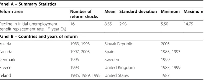
A decline in this indicator is assumed to signal a “reform”, which depending on the magnitude of the change can be fairly negligible or instead sizeable. In order to identify the effects of reform on aggregate unemployment, we focus on major reforms and identify reform shocksas follows. The standard deviation of the annual change in the benefit replacement rate indicator is calculated over all available observations. A major reform is then assumed to have been undertaken when the change in the policy indicator in a given year exceeds (minus) 2 standard deviations2. Because the criterion set to identify reform shocks is ultimately arbitrary, we perform sensitivity analysis to assess the robustness of the results to alternative thresholds (1.5 and 2.5 standard deviations). Table 1 presents for each sample country the reform shocks identified using this methodology, as well as basic summary statistics regarding the reform shocks. Over the sample, benefit reforms appear to have been carried out mainly in English-speaking countries (Australia, Canada, the United Kingdom, Ireland, New Zealand, and the United States) as well as in Nordic countries (Denmark, Norway, and Sweden).

2.2. Econometric approach

Based on the identification of reform shocks, a reform variable is constructed following the methodology outlined by Romer and Romer (2010) to estimate fiscal multipliers at various horizons based on measures of fiscal shocks. The following“reform variable”is constructed by country and year: i) when a reform shock has been identified for a particular country and year, the reform variable takes the value of the change in the associated policy indicator; ii) if no reform shock has been identified, the reform variable takes a zero value. Allowing the reform variable to take the value of the change in the underlying policy indicator results in a continuous variable that allows quantifying the

Table 1 The reform shocks: summary statistics and country details

Panel A–Summary Statistics

Reform area Number of

reform shocks

Mean Standard deviation Minimum Maximum

Decline in initial unemployment benefit replacement rate, 1styear (%)

16 8.55 2.93 5.50 14.75

Panel B–Countries and years of reform

Austria 1983, 1993 Slovak Republic 2005

Canada 1997, 2005 Spain 1985, 1993

Denmark 1995 Sweden 1999

Greece 1993 United Kingdom 1983, 1999

(4)

impact of reform shocks, which would not be possible by considering a simple dummy variable instead3. Relying on the constructed benefit reform variable, impulse responses to the reforms are then estimated for the aggregate employment rate. The employment rate is preferred over the unemployment rate in order to account for any offsetting unemployment and labor force participation effects – for instance, any reform-driven decline in unemployment could in principle be concomitant with a decline in labor force participation, resulting in a smaller gain or even a decline in the overall employment rate.

The estimation of IRFs is then based on the simple approach proposed by Jorda (2005). Concretely, the following cross country time-series equation is estimated for

eachof the five years (k= 1. . .5) after the occurrence of the reform shock,

Ei;tþkEi;t¼αkþ Xj¼5

j¼0

βk_;jΔEi;tjþθkreformi;tþ Xj¼5

j¼0

λh;k;jcrisish;k;tjþγi_;kþγt;kþεi;t;k;

ð1Þ

where Ei,tis the employment rate in country i at timet, reform is the benefit reform

variable (which, as explained above, is equal to the variation of the underlying policy indicator in case a reform has been identified and zero otherwise),crisishis a set of four

dummies taking value one if the country experienced respectively a bank crisis, a currency crisis, a debt crisis, or a recession, andγikandγtkare respectively country and time fixed effects. Five lags of the crisis dummies are introduced. The financial crisis dummies are taken from Laeven and Valencia (2008). The recession dummy is equal to one in years when real GDP growth is negative and zero otherwise.

The introduction of a dummy variable coding for recessions is justified by the finding that economic crises are major facilitators of the reform process (see e.g. Duval 2008). Because economic crises are also likely to affect the dependent variable while being correlated with the probability to observe a reform shock, not controlling for them in the regression would introduce an omitted variable bias. Reverse causality should not be an issue in this set-up provided reforms were not introduced in response to afuture

expectedchange in the (un)employment rate. Even if the latter condition were not met,

the political economy literature suggests certain reforms would typically be undertaken in response to a future crisis, i.e. to a decline–rather than an increase–in employment. Therefore any associated bias in the estimated coefficientsθkin Equation 1 would be in the direction of finding adverse short-term employment effects of reform. Yet, despite such (highly) hypothetical bias, the estimates presented in Section 3 below show in fact a beneficial short-term employment impact of reform.

(5)

by relaxing the threshold above which a major reform is identified, thereby increasing the number of shocks considered in the estimation. Our results are robust to this test. Robust standard errors are clustered at the country level. Parameter estimates of the autoregressiveβs, the fixed effectsγor the crisis dummies are of no particular interest for the analysis4.

The employment impact of benefit reform could potentially be weaker in depressed labor markets. Raising incentives for the unemployed to intensify job search and accept existing offers might be effective at increasing outflows from unemployment when the labor market is tight, but could become less effective when labor demand is particularly weak – which may happen if the monetary authority cannot respond to maintain full employment, as may be the case for a member country of a large monetary union or in a depressed economic situation where the zero-bound constraint on monetary policy becomes binding. In order to explore this possibility, the econometric analysis also assesses whether the impact of benefit reforms varies depending on the cyclical pos-ition of the economy. In practice, an indicator of the cyclical condpos-itions is interacted with the reform shock variable as follows:

Ei;tþkEi;t ¼αkþ

Xj¼5

j¼0

βkjΔEi;tjþθkreformitþδkreformitcycleitþρkcycleit

þX

j¼5

j¼0

λh;k;jcrisish;k;tjþγikþγtkþεitk:

ð2Þ

where cycleitis the cyclical position of the economy considered just prior to the

intro-duction of the reform and is measured by the OECD’s estimate of the unemployment gap. Because the latter is ultimately an unobserved variable subject to some degree of uncertainty, we regard this part of the analysis as more suggestive than fully conclusive.

3. Estimation results

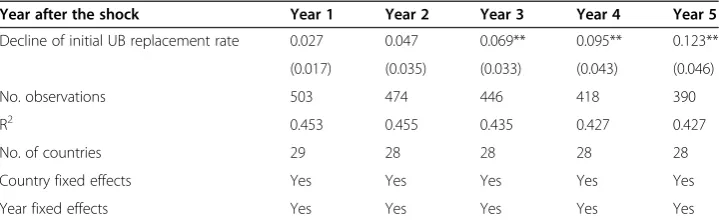
The estimation results are shown in Table 2. The employment rate impact of a reduction in the initial unemployment benefit replacement rate appears to materialize only grad-ually. The estimated effect becomes statistically significant only in the third year, and is still increasing into the fifth year. For example, a reduction in the initial unemployment benefit replacement rate of around 8 percentage points (corresponding to the median reform in the estimation sample) would translate into a 0.5 percentage point increase in the employment rate after three years and into an almost 1 percentage point

Table 2 Baseline estimation results

Year after the shock Year 1 Year 2 Year 3 Year 4 Year 5

Decline of initial UB replacement rate 0.027 0.047 0.069** 0.095** 0.123**

(0.017) (0.035) (0.033) (0.043) (0.046)

No. observations 503 474 446 418 390

R2 _0.453 _0.455 _0.435 _0.427 _0.427

No. of countries 29 28 28 28 28

Country fixed effects Yes Yes Yes Yes Yes

Year fixed effects Yes Yes Yes Yes Yes

(6)

increase after five years (Figure 1). The latter effect is comparable in magnitude to the steady-state impact estimated in Bassanini and Duval (2006), suggesting that it may take as much as five years on average for the full gains from benefit reform to materialize.

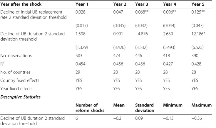
The generosity of unemployment insurance depends on both replacement rates and the duration of benefits. We hence extend the previous analysis by controlling the regression for the impact of reforms reducing the duration of unemployment benefits (Table 3). Following the approach in Nickell et al. (2005) and Bassanini and Duval (2009), the underlying benefit duration variable is computed indirectly as the ratio of (OECD measures of ) average replacement rates over a five-year unemployment spell to first-year replacement rates5. Bearing in mind that only six reform shocks are identified over the sample, results are qualitatively consistent with those reported above but the impact of benefit duration reforms seems to take more time to materialize, up to five years.

The empirical analysis suggests that the short-term impact of unemployment benefit reforms varies depending on the business cycle position (Table 4, Panel A). Evaluating the size of these interactions requires calculating marginal effects of reforms for differ-ent levels of economic activity (and their corresponding standard errors). Table 4, Panel B reports synthetic results on the employment impact of the unemployment benefit reform calculated at the minimum, median and maximum values of the unemployment gap. While the baseline analysis suggests that on average positive effects of this reform materialise quite rapidly, interacting the reform shock variable with the unemployment gap suggests that short-term gains are stronger during“good”times, and weaker–and in some cases even negative–during“bad”times. This finding is consistent with some micro-econometric evidence (Bover et al. 2002; Schmieder et al. 2012) which points to smaller disincentive effects from unemployment benefits – and therefore to smaller potential job search intensity and employment gains from benefit reform – in weak economic conditions. Taken at face value, the estimates imply that a median reduction

(7)

Table 3 The impact of benefit duration reforms

Decline of initial UB replacement rate 2 standard deviation threshold

0.028 0.047 0.068** 0.096** 0.125**

(0.017) (0.035) (0.032) (0.044) (0.047)

Decline of UB duration 2 standard deviation threshold

1.598 0.991 −4.876 2.630 12.186*

(1.329) (3.426) (3.532) (5.493) (6.525)

No. observations 503 474 446 418 390

R2 0.454 0.456 0.436 0.427 0.428

Country fixed effects YES YES YES YES YES

Year fixed effects YES YES YES YES YES

Descriptive Statistics

Number of reform shocks

Mean Standard

deviation

Minimum Maximum

Decline of UB duration 2 standard deviation threshold

6 −0,2 0.09 −0,13 −0.36

***, ** and * represent statistical significance at the 1%, 5% and 10% levels, respectively. Robust standard errors are in parentheses.

Table 4 The influence of economic conditions

Panel A_–Estimation results

Decline of initial UB replacement rate 0.025 0.047 0.075** 0.125** 0.165***

(0.016) (0.032) (0.030) (0.051) (0.052)

Unemployment Gap −0.194*** −0.666*** −1.221*** −1.711*** −2.000***

(0.061) (0.120) (0.179) (0.261) (0.329)

(Decline of initial UB replacement rate) × (Unemployment Gap)

0.002 0.011 0.029** 0.049*** 0.061***

(0.005) (0.011) (0.012) (0.018) (0.019)

No. observations 492 463 435 407 379

R2 0.482 0.523 0.553 0.590 0.613

Country fixed effects Yes Yes Yes Yes Yes

Panel B–Synthetic results of the employment impact of the UB reform at the minimum, median and maximum values of the unemployment gap (in percentage points)

Minimum 0.102 −0.201 −0.918 −1.559* −1.876**

(0.237) (0.479) (0.557) (0.778) (0.873)

Median 0.184 0.327 0.490** 0.819** 1.097***

(0.117) (0.228) (0.215) (0.364) (0.372)

Maximum 0.226 0.607 1.235*** 2.073*** 2.661***

(0.198) (0.435) (0.445) (0.687) (0.699)

(8)

in the initial unemployment benefit replacement rate would bring about a 0.5 percentage point employment gain after three years when the unemployment gap is at its median value of close to zero, but the same reform would not have any statistically significant effect for lower values of the initial unemployment gap and even bring significant employment losses in very depressed labor markets (Figure 2)6.

4. Sensitivity analysis

In order to assess the sensitivity of the baseline results, we perform the three following robustness checks:

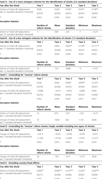
The use of alternative thresholds beyond which the change in a benefit replacement rate indicator is identified as a reform shock. In the baseline approach, a reform shock is identified when the benefit replacement rate indicator varies by more than two standard deviations of the annual variation calculated over all available observations. Here we test for the robustness of the baseline results when reducing or increasing the occurrence of reform shocks, i.e. by raising the stringency criterion used to identify them to 2.5 standard deviations or reducing it to 1.5 standard deviations. This comes across as considering “smaller” and “larger” reforms than in the baseline, respectively.

The introduction of “reverse” reforms, measured as large changes in the benefit replacement rate indicator in the opposite direction, as additional control variables7. The results from the baseline approach are based on regressions that ignore“reverse” reforms, which can be defined as a large increase in the benefit replacement rate. Insofar as large increases in benefit replacement rates reduce employment rates, omitting them from the regressions may lead to an overestimation of the positive effects of reforms. Instead of disentangling the effects of positive and negative reform shocks by including a new variable for reverse shocks, an alternative strategy is to

-2.5 -2 -1.5 -1 -0.5 0 0.5 1 1.5 2 2.5 3

0 1 2 3 4 5

Years after the shock

"good" times

"bad" times

Percentage points

(9)

specify a new reform shock variable including simultaneously positive and negative shocks.

The exclusion of the country fixed effects. Country fixed effects are aimed at controlling for country-specific trends in the employment rate, since the latter enters the equation in difference. Yet this empirical model might be incorrectly specified if unobserved heterogeneity between countries applies to the level rather than the growth rate of the employment rate, in which case a model without fixed effects would better capture the underlying dynamics. This is unlikely to be the case here since the country fixed effects are statistically significant in the baseline regressions. Nevertheless, as a robustness test, regressions are run without country fixed effects.

The baseline results appear to be robust to these robustness checks (Table 5).

Estimates obtained by reducing or alternatively, by increasing the number of re-form shocks (shocks identified respectively with a threshold of 2.5 standard devia-tions and with a threshold of 1.5 standard deviadevia-tions) are qualitatively similar to those obtained in the baseline (Panels A and B), although coefficients get more sig-nificant when the number of shocks considered is larger. Introducing “reverse” reforms in the regression (Panel C) barely modifies the estimates, suggesting that the effects of the unemployment benefit reform identified in the baseline approach are not overestimated due to the omission of increases in benefit replacement rates that may dampen labor market performance. Results from an alternative approach based on a single reform shock variable including positive and negative shocks are gener-ally less robust than those obtained when allowing the coefficient to differ between opposite-signed reforms (Table 5 Panel D). This suggests that the effects of policy changes are not symmetrical. Finally, results reported in Table 5, Panel E excluding country fixed effects are more significant than those obtained with country fixed effects, with positive effects of a decrease in the benefit replacement rates that may materialize from the first year.

5. Conclusion

(10)

Table 5 Sensitivity analysis

Panel A - Use of a more stringent criterion for the identification of shocks (2,5 standard deviation)

Decline of initial UB replacement rate 2.5 standard deviation threshold

0.026 0.036 0.054* 0.074* 0.106**

(0.019) (0.035) (0.031) (0.041) (0.043)

R2 _0.453 _0.455 _0.435 _0.426 _0.426

Descriptive Statistics Number of reform shocks Mean Standard deviation Minimum Maximum

11 9.84 2.65 −7 −14,75

Panel B - Use of a less stringent criterion for the identification of shocks (1.5 standard deviation)

0.038 0.063 0.093** 0.138** 0.171***

(0.023) (0.039) (0.043) (0.051) (0.051)

R2 0.454 0.456 0.436 0.429 0.429

23 7.34 3.068 −4 −14.75

Panel C - Controlling for“reverse”reform shocks

0.026 0.045 0.066* 0.094** 0.124**

(0.018) (0.036) (0.032) (0.043) (0.047)

Increase of initial UB replacement rate 2 standard deviation threshold −

0.008 −0.013 −0.016 −0.008 0.004

(0.019) (0.040) (0.042) (0.037) (0.040)

R2 0.453 0.456 0.436 0.427 0.427

16 8.55 2.93 −5.50 −14.75

Increase of initial UB replacement rate 2 standard deviation threshold

10 18.84 8.61 11.54 38.46

Panel D–Controlling for“reverse”reform shocks (single variable including two types of shocks)

Change of initial UB replacement rate 2 standard deviation threshold −

0.013 ₋0.022 ₋0.028 ₋0.029 ₋0.027

(₋1.06) (₋0.76) (₋0.84) (₋0.91) (₋0.77)

R2 _0.453 _0.455 _0.435 _0.426 _0.424

Change of initial UB replacement rate 2 standard deviation threshold

26 1.99 14.71 −14.75 38.46

Panel E - Excluding country fixed effects

0.044** 0.090*** 0.155*** 0.220** 0.283***

(0.017) (0.028) (0.046) (0.081) (0.094)

(11)

Endnotes 1

The existence of interactions between labor market institutions implies in particular that the adverse employment effects of high and long-lasting benefits can be mitigated and even possibly be fully offset by well-designed active labor market policies, along the lines of the Danish “flexicurity” model. For empirical evidence on such effect and on interactions be-tween labor and product market regulations more broadly, see Bassanini and Duval (2009).

2

A priori, one potential concern could be that some large unemployment benefit reforms may have been incremental in nature, and would therefore be missed by the criterion applied here. This is a feature which the empirical approach, which focuses on reform “shocks”, cannot fully capture. However, because any large but incremental reforms will be coded as non-reforms, the empirical results can only be“biased”against finding significant effects.

3

While our construction of the reform shock variables is inspired by Romer and Romer’s, it is worth underlying the differences between the two approaches. Romer and Romer (2010) use a vastnarrativerecord describing the motivation of tax changes from which the authors identify reforms that are not directly related with other develop-ments affecting output. In contrast to the narrative approach used by Romer and Romer, our identification strategy relies on the use of a threshold approach to identify major changes in the institutional variable. The impacts of these major shocks are then estimated against the scenario of either no reform or gradual reform.

4

An alternative to this econometric approach would have been to estimate one single auto regressive distributed lag (ARDL) specification and to derive IRFs from the estimated coefficients. This approach was initially proposed by Romer and Romer (1989, 2010), and it has been recently applied by Cerra and Saxena (2008) to assess the impact of financial crises on GDP growth. However, because IRFs are calculated recursively in this approach, they have been criticized for being sensitive to small specification errors that always exist in practice (Teulings and Zubanov 2010). Specifically, IRFs derived using an ARDL specification tend to be sensitive to the choice of the number of lags, and as a result can be unstable.

5

More precisely, this measure captures the extent to which unemployment benefits decline throughout the unemployment spell. In practice, it appears to vary between 0.2 and 1, where 1 indicates a situation where unemployment benefits do not decline during the period spent in unemployment.

Table 5 Sensitivity analysis(Continued)

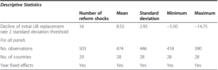
Descriptive Statistics

Number of reform shocks

Mean Standard

deviation

Minimum Maximum

16 8.55 2.93 ₋5.50 ₋14.75

For all panels

No. observations 503 474 446 418 390

(12)

6

The impact of the reform is found to be statistically insignificant for values of the unemploy-ment gap lower than−1.4 and significantly negative for values of the unemployment gap lower than−5.2 (the minimum level of the unemployment gap is equal to−6.8 in the sample).

7

Following the Romer and Romer (2010) approach used above, the associated variable is equal to this large change when it is observed and zero otherwise.

Competing interests

TheIZA Journal of Labor Policyis committed to the IZA Guiding Principles of Research Integrity. The authors declare that they have observed these principles.

Acknowledgements

We would like to thank Aleksandra Zdzienicka for her collaboration to this work. We thank one anonymous referee, and the editor, Juan Francisco Jimeno. All remaining errors are ours.‘We would like to thank Aleksandra Zdzienicka for her collaboration to this work as well as Jorgen Elmeskov and Jean-Luc Schneider for providing useful comments during all the process. The authors are also grateful to one anonymous referee, and the editor, Juan Francisco Jimeno for their suggestions. Thanks also to participants to OECD Economics Department seminars, European Central Bank workshop and Tallinn University seminar. All remaining errors are ours.’

Responsible editor: Juan Francisco Jimeno

Author details

1_{OECD Economics Department Paris, France.}2_{IMFWashington D.C, USA.}

Received: 7 November 2012 Accepted: 20 December 2012 Published: 27 December 2012

References

Bassanini A, Duval R (2006) Employment patterns in OECD countries: reassessing the role of policies and institutions. OECD Economics Department Working Papers No. 486, OECD Publishing

Bassanini A, Duval R (2009) Unemployment, institutions, and reform complementarities: re-assessing the aggregate evidence for OECD countries. Oxford Rev Econ Policy 25:40–59

Blanchard O, Tirole J (2008) The joint design of unemployment insurance and employment protection: a first pass. J Eur Econ Assoc 6:45–77

Bover O, Arellano M, Bentolila S (2002) Unemployment duration, benefit duration and the business cycle. Econ J 112:223–265 Cacciatore M, Duval R, Fiori G (2012) Short-term gain or pain? A DSGE model-based analysis of the short-term effects of

structural reforms in labor and product markets. OECD Economics Department Working Papers No. 948, OECD Publishing

Card D (1990) The impact of the Mariel boatlift on the Miami labor market. Ind Labor Relat Rev 43:245–257 Card D, Krueger A (1994) Minimum wages and employment: a case study of the fast-food industry in New Jersey and

Pennsylvania. Am Econ Rev 84:774–775

Cerra V, Saxena SC (2008) Growth dynamics: the myth of economic recovery, American Economic Review. Am Econ Assoc 98(1):439–457

Duval R (2008) Is there a role for macroeconomic policy in fostering structural reforms? Panel evidence from OECD countries over the past two decades. Eur J Polit Econ 24:491–502

Eggertsson G (2010) The paradox of toil. Staff Reports No. 433, Federal Reserve Bank of New York

Everaert L, Schule W (2008) Why it pays to synchronize structural reforms in the euro area across markets and countries. IMF Staff papers, vol. 55(2) Palgrave Macmillan,pp 356–366

Gomes S, Jacquinot P, Mohr M, Pisani M (2011) Structural reforms and macroeconomic performance in the euro area countries: a model-based assessment. Working Paper Series No. 1323, European Central Bank

Greene W (2000) Econometric analysis. Prentice Hall edition, Englewood Cliffs, New Jersey

Jorda O (2005) Estimation and inference of impulse responses by local projections. Am Econ Rev 95:161–182 Laeven L, Valencia F (2008) Systemic banking crises: a new database. IMF Working Paper No. 08/224, International

Monetary Fund

Layard R, Nickell S, Jackman R (1991) Unemployment: macroeconomic performance and the labor market. Oxford University Press, Oxford

Nickell S (1981) Biases in dynamic models with fixed effects. Econometrica 49:1417–1426

Nickell S, Nunziata L, Ochel W (2005) Unemployment in the OECD since the 1960s: what do we know? Econ J 115:1–27 Pissarides C (2000) Equilibrium unemployment theory. MIT Press, Cambridge, Massachusetts

Romer CD, Romer DH (1989) Does monetary policy matter? A new test in the spirit of Friedman and Schwartz NBER Chapters. In: NBER Macroeconomics Annual 1989, Vol. 4. National Bureau of Economic Research, Inc, pp 121–184 Romer C, Romer D (2010) The macroeconomic effects of tax changes: estimates based on a new measure of fiscal

shocks. Am Econ Rev 100:763–801

Schmieder J, von Wachter T, Bender S (2012) The effects of extended unemployment insurance over the business cycle: evidence from regression discontinuity estimates over twenty years. Q J Econ 127:701–752

Teulings CN, Zubanov N (2010) Is economic recovery a myth? Robust estimation of impulse responses. CEPR Discussion Papers No. 7800

doi:10.1186/2193-9004-1-12