O R I G I N A L A R T I C L E
Open Access
Do non-wage cost rigidities slow down
employment? Evidence from Turkey
Sinem H Ayhan
Correspondence:
haticesinem.ayhan2@unibo.it Department of Economics, University of Bologna, Bologna, Italy
Abstract
This paper examines the role of non-wage cost rigidities in slowing down employment creation by assessing the effect of a policy aimed at fostering employment for women and young men introduced in Turkey in 2008. Exploiting a difference-in-difference-in differences strategy, I assess the employment effect of the reduction in the employer contribution share of the social security premiums. The results, net of the recent crisis effect, suggest a positive effect of the reduction in non-wage costs on employment creation for the targeted group (women) shortly after the announcement of the policy.
JEL Classification: C31; J08; J21; J32
Keywords: Social security contribution cut; Employment creation; Policy evaluation
1 Introduction
The employment rate in Turkey, fluctuating between 40%–50%, has been ranking the lowest in Europe for the last decade. Even Poland and Romania, amongst the lowest rank-ing EU countries, have an employment rate more than 15 percentage points higher than Turkey, as displayed in Table 11. The divergence in employment rate between Turkey and the EU is mainly because of the dramatically low rate of female employment in Turkey. As of 2007 only 21% of women were employed in Turkey, corresponding to one third of the EU average.
Reasons behind the divergence in employment performances among countries have been central to the literature in labor economics. A number of national and international surveys point at high non-wage costs, particularly high social security contributions in Turkey that create a burden on employers, and this in turn discourages employment creation in the formal sector while encouraging informal employment (OECD 2007; TCEA 2006; World Bank 2006). This view, also shared by the Turkish policy makers, was embodied in a policy intervention legislated in May 2008. The law prescribed a cut (up to 100%) in social security contributions borne by employers who hired young men (aged 18 to 29 years) and women (aged over 18 years) between July 1st, 2008 and June 30th, 2010. The main goal of this paper is to conduct a micro-econometric analysis to evaluate the effectiveness of this policy in creating formal employment for the tar-geted group (women), something that, to the best of my knowledge, has not been done yet.
© Ayhan; licensee Springer. This is an Open Access article distributed under the terms of the Creative Commons Attribution License (http://creativecommons.org/licenses/by/2.0), which permits unrestricted use, distribution, and reproduction in any medium, provided the original work is properly cited.
Table 1 Employment rates by the selected countries (as a share of working age population, aged 15–64)
Total Men Women
1995 2007 1995 2007 1995 2007
Bulgaria 50.4 61.7 54.7 66.0 46.3 57.6
Estonia 64.6 69.4 69.6 73.2 60.3 65.9
Latvia 59.9 68.3 65.1 72.5 55.1 64.4
Lithuania 62.3 64.9 66.2 67.9 58.6 62.2
Poland 58.9 57.0 66.8 63.6 51.3 50.6
Romania 65.4 58.8 71.9 64.8 59.1 52.8
Slovakia 60.6 60.7 67.8 68.4 53.5 53.0
EU-15 60.1 66.8 70.5 74.2 49.7 59.5
EU-27 60.7 65.3 70.0 72.5 51.4 58.2
Turkey 50.0 41.5 71.8 62.7 28.7 21.0
Source:Eurostat (2012) for EU countries; Turkstat (2012) for Turkey.
Note: The earliest data available for Poland, Romania and EU-27 is 1997, for Estonia, Latvia and Lithuania is 1998, and for Bulgaria is 2000.
Employment subsidy policies in the form of social security contribution cuts have taken place in several countries mostly in the northern Europe such as France (e.g. Kramarz and Philippon (2001)), Belgium (e.g. Goos and Konings (2007)), Sweden (e.g. Bennmarker et al. (2008); Egebark and Kaunitz (2010)) and Finland (e.g. Huttunen et al. (2010)) over the last two decades. Chile (e.g. Gruber, (1997)) and Turkey (e.g. Betcherman et al. (2010); Uysal (2013)) are the only known examples of developing countries where employment subsidies have empirically been analyzed. The employment subsidies generally target disadvantaged groups (e.g. low-wage workers, the young or the old), certain sectors or geographic locations rather than being applied to all workers and/or to all establishments. The availability of certain target groups enables the researchers to analyze the effective-ness of employment subsidies through difference-in-differences and/or triple difference strategy. The studies have mostly found little or no evidence of an employment effect of labor tax reduction with a few exceptions (i.e. Betcherman et al. (2010); Goos and Konings (2007); Uysal (2013))2.
Turkish non-wage subsidy policy in 2008 and employment creation. There is only little empirical research on developing countries in the field of employment subsidies. The existing literature, moreover, does not focus on the total number of employ-ment positions created by the policy that this paper intends to explore by using flow data.
The paper is organized as follows: Section 2 documents an overview of non-wage cost rigidities in the Turkish labor market and then introduces the policy of interest. Section 3 describes the data and the technique used to construct flow data. The identifi-cation strategy is discussed in Section 4, and estimation results are presented in Section 5. Section 6 concludes, and finally the appendix where the regressions and all the figures and tables are presented is provided.
2 An overview of non-wage costs in Turkey
Various factors could play a role in explaining the relatively poor employment per-formance of the Turkish labor market. One convincing explanation for the low rate of employment in the formal sector alongside the large size of informal employment (accounting for 45% of total employment) could be related to the factors increasing the cost of labor, apart from wage cost, given that the only labor cost employers have to bear in the informal sector is wage cost3.
The so-called “non-wage costs” refer to the part of total labor cost that is not directly related to actual working hours, including income tax on wages, employers’ and employees’ contributions to the social security premiums and unemployment insurance fund. These costs create a wedge between the cost the employer has to bear for hiring an employee and the wage received by the employee. As the wedge gets wider, the labor cost incurred by employers increases and employers become less willing to hire new workers in the formal sector. A widely used indicator to measure the weight of non-wage costs istax wedge. It is calculated as the ratio of income taxes plus employers’ and employees’ social security contributions (SSC) to total labor cost. The largest portion of the financial burden of labor taxes is incurred by employers in the majority of the OECD countries, including Turkey Organisation for Economic Co-operation and Development (2010).
in employers’ SSC. An evaluation of this regulation constitutes the main interest of this paper.
2.1 The 2008 employment package in Turkey
In response to high non-wage costs in Turkey, the policy makers introduced a law also known as “employment package” in May 2008. The package basically provides an exemption for employers from paying SSC with the intent of creating new employment for women (aged over 18 years) and young men (aged between 18 and 29). The exemption would gradually be phased out over a 5-year period. More specifically, the Unemploy-ment Insurance Fund would pay out 100% of employers’ SSC for the first year, 80% for the second year, 60% for the third year, 40% for the fourth year and 20% for the fifth year.
Employers can benefit from this subsidy if, and only if, the individuals they hire from the target group in any period between July 1st, 2008 and June 30th, 2010 are de facto employed within one year following the effective date of the regulation and in addition to the average number of previously registered insured workers having been declared in the one-year period preceding the effective date of this regulation (Law No. 5763 (2008)). The law also provides that the newly hired workers shall not be included among the previously registered insured workers in the six-month period preceding the effective date of the regulation. In order to avoid benefiting from the subsidy without creating new employment, the law excludes circulation of workers within sub-companies of the same employer; switching workers between direct or indirect partnerships, and also the situations in which an employer closes his company, opens another one and transfers his workers from the old to the new one.
In fact, the employment package that came into effect on 1 July 2008 was initially designed for one year. However, after the global economic crisis hit the Turkish labor market, a second employment package, extending the duration of the incentives for one more year, was introduced in order to alleviate the unfavorable impacts of the crisis on the effectiveness of the policy Law No. 5838 (2009). Likewise, to overcome the detrimental effects of the crisis on the labor market, similar employment incentives were introduced in August 2009 Uysal (2013). These incentives, regulated under a provisional article added to the Unemployment Insurance Law no. 4447, were provided for all new hirings, regardless of gender and age, for a six-month period. As stated by Uysal (2013), these additional incentives could mitigate the effectiveness of the policy of interest that targeted only female and young male employment. The potential effects of the other employ-ment incentives on my analysis will be touched on later, in Section 5 while discussing the estimation results.
3 Data and descriptive statistics
data, it is possible for the policy effect to be estimated by each quarter within the policy period, which will be further discussed in the following section. This will enable us to address the concerns raised by Uysal (2013), in that, to characterize whether the policy effect dies away after August 2009 probably because of the other employment incentives that were enacted meanwhile (as mentioned in Section 2.1).
Labor supply, constituting the outcome variable of this analysis, can be measured either through static variables such as annual working hours and employment probabilities or through flow variables such as transitions between labor market states. These states are conventionally defined as employment, unemployment and non-participation. The literature related to flow analysis focuses on two different kinds of transitions: worker and job flows. The latter measures whether a new position has been created or destroyed by a firm rather than the changes in the labor market status of the worker which is captured by the former measure Davis et al. (2006). Basically, job flows are measured on the basis of establishment or firm level data4, whereas worker flows are measured on the basis of individual or household level data5. A flow analysis is considered more appropriate for the aim of this paper that is to evaluate the effectiveness of the policy in creating new employment, which is unlikely to be captured by static variables. Moreover, the data set used in this paper, namely a household labor force survey makes a flow analysis based on worker transitions rather appropriate. Although the survey does not include a panel com-ponent, the retrospective questions in the questionnaire such as the labor market status one year before the survey enable us to track individuals in two consecutive survey peri-ods. These retrospective questions are exploited to construct the flow data. For instance, flows from employment to unemployment include the respondents who report their cur-rent status as unemployed while their recalled status one year prior to the survey was employed6.
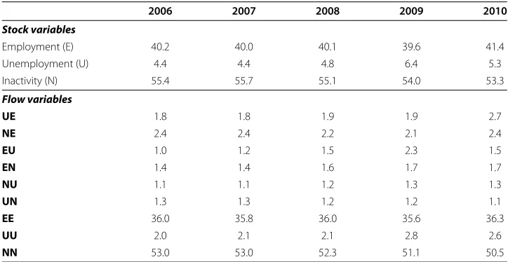
New employment creation, defined as the difference between hirings and separations, is calculated by subtracting flows into employment from flows out of employment Davis et al. (2006). Following Bell and Smith (2002) and Elsby et al. (2011),hiringis defined as the sum of flows from unemployment to employment and flows from inactivity to employment, whereasseparationis equal to flows from employment to unemployment plus flows from employment to inactivity. Flows between unemployment and inactivity are also examined in order to capture a potential change in the job searching behavior of individuals. Table 2 presents flow rates for nine possible transitions between and within labor market states of employment (E), unemployment (U) and inactivity(N). The flow variables displayed in the table are denoted by two letters, representing the initial and arrival labor market states, respectively.
Table 2 Rates of stock and flow variables (as a percentage of population aged 15 and over)
2006 2007 2008 2009 2010
Stock variables
Employment (E) 40.2 40.0 40.1 39.6 41.4
Unemployment (U) 4.4 4.4 4.8 6.4 5.3
Inactivity (N) 55.4 55.7 55.1 54.0 53.3
Flow variables
UE 1.8 1.8 1.9 1.9 2.7
NE 2.4 2.4 2.2 2.1 2.4
EU 1.0 1.2 1.5 2.3 1.5
EN 1.4 1.4 1.6 1.7 1.7
NU 1.1 1.1 1.2 1.3 1.3
UN 1.3 1.3 1.2 1.2 1.1
EE 36.0 35.8 36.0 35.6 36.3
UU 2.0 2.1 2.1 2.8 2.6
NN 53.0 53.0 52.3 51.1 50.5
Source: Author’s own calculations based on micro data from Turkstat.
Likewise, the separation rate (the sum of EU and EN) has also seen more than one per-centage point increase between 2007 and 2009 probably because of the crisis effect, and then it has started to decrease with the recovery from the crisis.
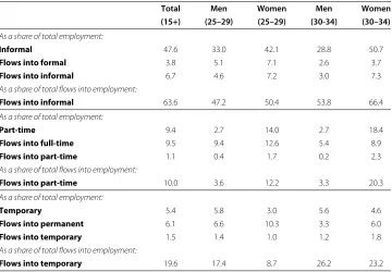
The policy could also have an impact on within-employment transitions through for-malization of the existing job and/or by changing the type of employment (i.e. full-/ part-time versus permanent/temporary)7. However, there is no information in the survey about the social security coverage and employment type of the previous year’s job. There-fore, it is impossible to examine the employment-to-employment transitions in these respects. Nevertheless, it is feasible to track what kind of jobs the individuals transit into without knowing the type of job they were working during the previous year. As Table 3 presents, 47% of the employed people in the sample do not have a social security cov-erage as of 2007, and transitions into employment are more likely to be into informal employment which account for 63% of total flows into employment. Informality is more common among female workers relative to their male counterparts, especially among women aged 30 to 348. In parallel, the incidence of transiting into informal employment is higher among women.
On the other hand, atypical employment arrangements such as part-time and tempo-rary employment do not represent a considerable proportion in total employment. As displayed in Table 3, only one tenth of the employed people work in a part-time job while the remainder have a full-time job. Similarly, only 5% of the employed hold temporary contracts. Part-time employment is higher by far among women for both age groups, whereas it is the reverse as regards to temporary employment. The low incidence of atypi-cal employment arrangements is accompanied by a larger share of transitions into regular jobs. As a share of the total flows into employment, flows into full-time and permanent employment account for 90% and 80%, respectively9.
4 Identification strategy
Table 3 Informal and atypical employment, 2007
Total Men Women Men Women
(15+) (25–29) (25–29) (30-34) (30–34) As a share of total employment:
Informal 47.6 33.0 42.1 28.8 50.7
Flows into formal 3.8 5.1 7.1 2.6 3.7
Flows into informal 6.7 4.6 7.2 3.0 7.3
As a share of total flows into employment:
Flows into informal 63.6 47.2 50.4 53.8 66.4
As a share of total employment:
Part-time 9.4 2.7 14.0 2.7 18.4
Flows into full-time 9.5 9.4 12.6 5.4 8.9
Flows into part-time 1.1 0.4 1.7 0.2 2.3
As a share of total flows into employment:
Flows into part-time 10.0 3.6 12.2 3.3 20.3
As a share of total employment:
Temporary 5.4 5.8 3.0 5.6 4.6
Flows into permanent 6.1 6.6 10.3 3.3 6.0
Flows into temporary 1.5 1.4 1.0 1.2 1.8
As a share of total flows into employment:
Flows into temporary 19.6 17.4 8.7 26.2 23.2
Source: Author’s own calculations based on micro data from Turkstat.
and after the policy period. This allows using difference-in-differences (DD) strategy to analyze the employment effect of the policy on women and young men. Recalling the policy design described in Section 2.1., the treatment group (those targeted by the policy) could be selected from among men aged 20-29 and women over 18 years old, and the control group (those not targeted by the policy) could be selected from among men aged over 29 years. Given that the data do not provide exact ages of the individuals, but 5-year age brackets, in order to explore the causal effect of the policy on employment creation for young men, the relative outcomes of men aged 25 to 29 are compared with those of men aged 30 to 34 between before and after the policy introduction10. Similarly, to evaluate the employment effect of the policy on women, the relative outcomes of women aged 30 to 34 are compared with those of men of the same age group between before and after the policy introduction11.
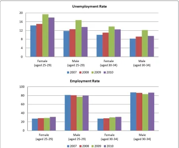
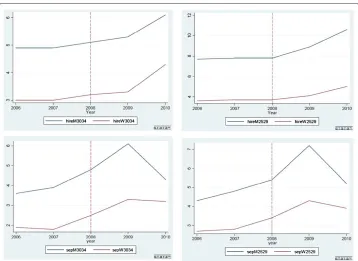
Figure 1 Employment rates of the treatment and control groups between 2000 and 2010. Source: Turkstat (2012).
between 2003 and 2008, as shown in Figure 113. In relation to this, I test the difference in the mean of relevant observable characteristics between the treatment and control group. The results support the hypothesis of no significant difference between the two groups.
One potential problem in this analysis would be if employers had expected the enact-ment of the policy and strategically delayed hiring new workers or fired the existing workers in the control group until the law was introduced with the intent of benefiting from the incentives. However, it is needless to worry about such a problem given that the policy was announced only two months before the implementation period, and benefiting from the incentives is conditional on additional hiring as mentioned before.
The DD strategy would have been appropriate to analyze the causal effect of the pol-icy intervention if the crisis had not affected the labor market outcomes of the subgroups differently. Given the differential effect of the crisis across treatment and control groups, as can be seen in Figure 2, the policy evaluation through DD strategy is potentially con-founded by the crisis effect. In order to rule out the possible confounding effects of the crisis, difference-in-difference-in-differences (DDD) strategy is exploited. This strategy is advantageous over a double difference analysis in policy evaluation, especially in the presence of an economic shock which could play a determining role in the effective-ness of the policy. Technically speaking, DDD strategy requires three dimensions to be implemented, which are age, gender and time in this context. Since the policy of interest targets all women over 18 years old, it is unlikely to use a group of women as a control group and accordingly to conduct a DDD analysis for evaluating the policy effect on men. Therefore, the evaluation based on DDD strategy is confined to the effect of the policy on women.
Figure 2 Unemployment and employment rates of treatment and control groups between 2007 and 2010.Source: Turkstat (2012).
30 to 34 under the assumption that both age groups have been affected by the crisis in a similar way.
The validity of this last assumption is tested in two steps. The first step is to test whether there is an age effect. To do this, a comparison is made in the relative out-comes of women aged 30 to 34 with their younger counterparts aged 25 to 29 between two periods before the policy intervention. Finding a statistically significant estimate of the coefficient of the interaction term would suggest the existence of an age effect, which would violate the assumption unless the age effect is the same for both gen-ders. The second step is to test whether the age effect is the same for women and men. To this end, the DDD analysis is replicated for the pre-policy period. If the null hypothesis that the coefficient estimate(s) of the triple interaction term are significantly different from zero is not rejected, it would imply that a comparison between two age cohorts would eliminate the differential crisis effect even if there is evidence of age effect, and so the identifying assumption would hold. In such a scenario, the second step test would be sufficient to prove the validity of the assumption. Given that no sig-nificant estimate was found in either step, the first step results are not presented for sake of brevity. The placebo test results are discussed in more detail in the following section.
out with the passing of time. In order to see whether the policy effect is quarter- and/or year-specific, three specifications are estimated based on the empirical strategy just out-lined above. First, the policy effect is imposed to be constant across quarters over the period. More specifically, there is no allowance for quarter and year specific dummies, and the comparison is between the entire period after the policy introduction and the entire period before the policy. This specification is called “period specific” policy effect. Next, the policy effect is imposed to be constant across quarters within a year, but allowing for variation between years by introducing year specific dummies for the policy period. This specification enables the estimation of the policy effect for each year over the policy period. Thirdly, an allowance is made for heterogeneous policy effect across quarters by including year specific quarter dummies. This time the comparison is between each quarter within the policy period and the entire period before the policy intervention. This most flexible specification provides separate estimates of the policy effect for each quarter over the policy period15. Furthermore, each quarter within the policy period is compared to the corresponding quarter in the pre-policy period in order to test the role of seasonality in policy effectiveness.
5 Results
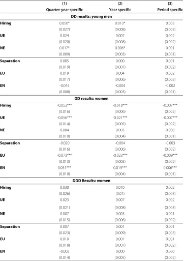
Table 4 presents the aggregate effect of the policy over the period. In fact, the same parameter is estimated in each column of the table, however, each column represents a different specification changing depending on the restriction imposed, as described in the previous section. The estimation results presented in this and in the following tables include all the control variables (i.e. completed years of schooling and marital sta-tus of the individuals, number of children in the household and a variable for urban/rural divide) in levels and of their interactions, although adding control variables does not change the significance of the results, but the precision of the estimates. The standard errors displayed in the tables arebootstrapstandard errors stratified at gender and age level16.
According to the DD estimation results displayed in the top and middle panels of Table 4, the probability of being hired for men aged 25 to 29 increased significantly above that for men aged 30 to 34 after the policy introduction, whereas a negative change was observed in the probability of being hired for women aged 30 to 34 relative to men of the same age group. The estimated negative effect of the policy on women could be attributable to the inability of the DD strategy in eliminating the differential effect of the crisis on different genders. That the negative and significant estimate obtained from the DD strategy turns into positive after canceling out the crisis effect implies the confounding role of the crisis in evaluating the policy.
Table 4 Aggregate effect of the policy over the period
(1) (2) (3)
Quarter-year specific Year specific Period specific DD results: young men
Hiring 0.050* 0.013* 0.003
(0.027) (0.008) (0.003)
UE 0.024 0.007 0.002
(0.020) (0.008) (0.002)
NE 0.017* 0.006* 0.001
(0.009) (0.003) (0.001)
Separation 0.005 0.000 0.001
(0.019) (0.007) (0.002)
EU 0.019 0.004 0.002
(0.017) (0.006) (0.002)
EN -0.014 -0.004 -0.002
(0.008) (0.003) (0.001)
DD results: women
Hiring -0.052*** -0.018*** -0.007***
(0.016) (0.006) (0.002)
UE -0.056*** -0.021*** -0.007***
(0.014) (0.005) (0.002)
NE 0.004 0.003 0.000
(0.010) (0.004) (0.001)
Separation -0.020 -0.004 -0.003
(0.016) (0.006) (0.002)
EU -0.073*** -0.023*** -0.009***
(0.013) (0.005) (0.002)
EN 0.051*** 0.019*** 0.006***
(0.010) (0.004) (0.001)
DDD Results: women
Hiring 0.030 0.010 0.002
(0.026) (0.01) (0.003)
UE 0.023 0.007 0.002
(0.021) (0.008) (0.003)
NE 0.007 0.003 0.001
(0.015) (0.006) (0.002)
Separation 0.007 0.001 0.001
(0.023) (0.009) (0.003)
EU 0.010 0.001 0.001
(0.018) (0.007) (0.002)
EN -0.003 0.000 0.000
(0.014) (0.005) (0.002)
Notes: (1) Bootstrap standard errors with 1000 replications are in parenthesis (*** p<0.01, ** p<0.05, * p<0.1) (2) Number of observations for the three specifications in the upper, middle and below panels are 144954, 147534 and 305590, respectively.
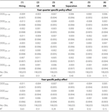
Table 5 Placebo test results for the DDD estimation
(1) (2) (3) (4) (5) (6)
Hiring UE NE Separation EU EN
Year-quarter specific policy effect
DDDQ3−06 -0.009 -0.003 -0.007 0.006 0.000 0.006
(0.007) (0.006) (0.004) (0.006) (0.005) (0.004)
DDDQ4−06 -0.013 -0.005 -0.008 -0.005 -0.008 0.003
(0.008) (0.006) (0.005) (0.006) (0.005) (0.004)
DDDQ1−07 -0.002 0.001 -0.003 0.000 -0.003 0.004
(0.008) (0.006) (0.005) (0.006) (0.005) (0.004)
DDDQ2−07 -0.011 -0.004 -0.007 -0.003 -0.002 -0.001
(0.008) (0.006) (0.005) (0.006) (0.005) (0.004)
DDDQ3−07 -0.003 0.002 -0.004 0.007 0.000 0.007
(0.008) (0.006) (0.005) (0.006) (0.005) (0.005)
DDDQ4−07 -0.002 0.000 -0.002 -0.002 -0.005 0.002
(0.008) (0.006) (0.005) (0.006) (0.005) (0.004)
DDDQ1−08 0.007 0.011 -0.005 0.002 0.000 0.002
(0.007) (0.007) (0.005) (0.007) (0.005) (0.004)
DDDQ2−08 -0.005 0.001 -0.006 -0.003 -0.001 -0.003
(0.008) (0.006) (0.005) (0.007) (0.005) (0.004)
No. Obs. 190,035 190,035 190,035 190,035 190,035 190,035
R2 0.63 0.51 0.28 0.40 0.33 0.15
Year specific policy effect
DDD2006 -0.011 -0.004 -0.007 0.001 -0.004 0.005
(0.007) (0.005) (0.005) (0.005) (0.004) (0.003)
DDD2007 -0.004 0.000 -0.004 0.000 -0.002 0.003
(0.005) (0.004) (0.003) (0.004) (0.003) (0.003)
DDD2008 0.001 0.006 -0.005 -0.001 -0.001 0.000
(0.006) (0.005) (0.004) (0.005) (0.004) (0.003)
No. Obs. 190,035 190,035 190,035 190,035 190,035 190,035
R2 0.63 0.51 0.28 0.40 0.32 0.15
Robust standard errors in parenthesis (*** p<0.01, ** p<0.05, * p<0.1).
specification which imposes constant policy effect across quarters, the probability of being hired for a woman aged 30 to 34 increased by 0.2% relative to a man of the same age group after the policy introduction. The same probability increased by 1% as for the less restricted specification which allows the policy effect to vary between years,
0.0 10.0 20.0 30.0 40.0 50.0 60.0
Total Men
aged 25-29
Men aged 30-34
Women aged 25-29
Women aged 30-34
Services Industry Agriculture Construction
and by 3% as for the most flexible specification which allows for variation across quar-ters. However, neither the estimates of the variablehiring nor the variable separation are statistically significant as far as the aggregate effect of the policy over the period is concerned.
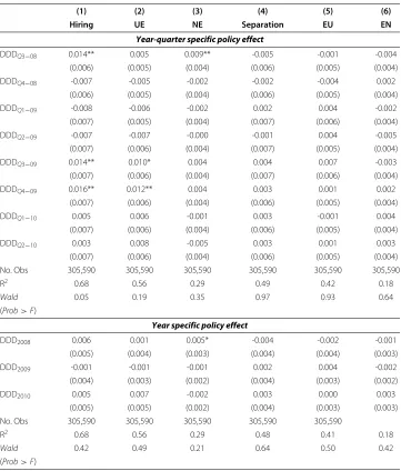
There may be some quarters where the policy is effective while in other quarters the estimated policy effect could be null, thus aggregating over the policy period would make the estimates statistically insignificant. The validity of this hypothesis was checked through the Wald test and evidence of heterogeneous policy effect across quarters was discovered, as presented in Table 6. The estimation results reported in the table point out that the disaggregation of the policy effect by quarter yields positive and statistically significant city of being hired for women aged 30 to 34 above men of the same age group increased by 1.4% in the third quarters of 2008 and 2009, and by 1.6% in the fourth quar-ter of 2009, afquar-ter removing the crisis effect17. Moreover, the positive effect of the policy
Table 6 DDD estimation results
(1) (2) (3) (4) (5) (6)
Hiring UE NE Separation EU EN
Year-quarter specific policy effect
DDDQ3−08 0.014** 0.005 0.009** -0.005 -0.001 -0.004
(0.006) (0.005) (0.004) (0.006) (0.005) (0.004)
DDDQ4−08 -0.007 -0.005 -0.002 -0.002 -0.004 0.002
(0.006) (0.005) (0.004) (0.006) (0.005) (0.004)
DDDQ1−09 -0.008 -0.006 -0.002 0.002 0.004 -0.002
(0.007) (0.005) (0.004) (0.007) (0.006) (0.004)
DDDQ2−09 -0.007 -0.007 -0.000 -0.001 0.004 -0.005
(0.007) (0.006) (0.004) (0.007) (0.005) (0.004)
DDDQ3−09 0.014** 0.010* 0.004 0.004 0.007 -0.003
(0.007) (0.006) (0.004) (0.007) (0.006) (0.004)
DDDQ4−09 0.016** 0.012** 0.004 0.003 0.001 0.002
(0.007) (0.006) (0.004) (0.006) (0.005) (0.004)
DDDQ1−10 0.005 0.006 -0.001 0.003 -0.001 0.004
(0.007) (0.006) (0.004) (0.006) (0.005) (0.004)
DDDQ2−10 0.003 0.008 -0.005 0.003 0.001 0.003
(0.007) (0.006) (0.004) (0.006) (0.005) (0.004)
No. Obs 305,590 305,590 305,590 305,590 305,590 305,590
R2 0.68 0.56 0.29 0.49 0.42 0.18
Wald 0.05 0.19 0.35 0.97 0.93 0.64
(Prob>F)
Year specific policy effect
DDD2008 0.006 0.001 0.005* -0.004 -0.002 -0.001
(0.005) (0.004) (0.003) (0.004) (0.004) (0.003)
DDD2009 -0.001 -0.001 -0.001 0.002 0.004 -0.002
(0.004) (0.003) (0.002) (0.004) (0.003) (0.002)
DDD2010 0.005 0.007 -0.002 0.003 0.000 0.003
(0.005) (0.005) (0.002) (0.004) (0.003) (0.003)
No. Obs 305,590 305,590 305,590 305,590 305,590
R2 0.68 0.56 0.29 0.48 0.41 0.18
Wald 0.42 0.49 0.21 0.64 0.50 0.42
(Prob>F)
on the variable hiring is mostly attributable to the flows from unemployment rather than those from inactivity, which is in accordance with the transition statistics presented in Table 2.
According to the estimation results reported in the tables, the coefficient estimates of the variableseparationare always statistically insignificant. This is actually in line with the expectation given that the eligibility for the subsidy is on the condition of hiring new employees in addition to the average number of registered workers declared in the pre-vious year. This condition rules out the possibility that employers fire an existing worker and hire a new one at the end of the first year to benefit from the full subsidy. Neverthe-less, both employment creation and destruction effects of the policy are estimated so as to measure net employment growth.
What could be the underlying reasons behind the significant policy effect in some quarters along with insignificant effect in the others? First, a check was made whether seasonality matters in characterizing the policy effect by introducing non-year specific quarter dummies in the interaction term. In particular, each quarter over the policy period is compared with the same quarter before the policy intervention. For instance, the third quarter after the policy period (of 2008 and 2009) is compared with the third quarter before the policy period (of 2006 and 2007). The results indicate no evidence of seasonality in the sense that the coefficients of the interaction terms were found sta-tistically insignificant. In fact, there is one evident explanation for the quarter-specific pattern in the policy effect. As mentioned in Section 2.1, the policy announced in May 2008 was initially designed for one year. After the economic crisis hit the labor market by the third quarter of 2008, the government decided to extend the policy period for one more year, and the statistically significant estimates in 2009 are detected precisely in quar-ters at the beginning of the second implementation year of the policy. As proposed by Uysal (2013), the reason why the policy effect dies out by the end of 2009 could be related to the introduction of new employment incentives provided for all new employment creation18.
Relying on the coefficient estimates in Table 6, further light will be shed on how much new employment was created by the policy. Given that new employment is defined as the difference between total hirings and separations, the relevant question is which aggregation level is proper for calculating total hirings and separations. Since the main interest of this study is to explore the causal effect of the policy on the treated, hiring and separation are aggregated by multiplying the corresponding probability with the number of women aged between 30 and 34 years (treated group) in the policy period. Focusing on the quarters in which there is evidence of significant policy effect, it was established that the policy created 92 new employment positions for women aged between 30 to 34 years in the third quarter of 2008, 54 positions in the third quarter of 2009 and 63 positions in the fourth quarter of 2009. This amounts to totally 209 new employment positions, accounting for 1.4% of the number of women in the relevant age group in the sample. Remarkably these magnitudes are similar to the employment gains reported by Uysal (2013) using descriptive statistics.
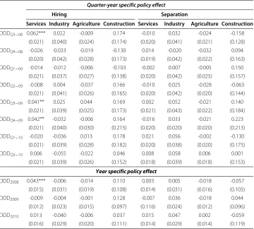
and construction sectors account for less than one fifth of the female employment. To disaggregate the policy effect by sector, the data are stratified by four main sectors; ser-vices, industry, agriculture and construction. The estimation results presented in Table 7 suggest that the probability of being hired for women aged 30 to 34 in the services sec-tor increased by 6.2% in the third quarter of 2008, 4.1% in the third quarter of 2009 and 4.2% in the fourth quarter of 2009 relative to their male counterparts of the same age cohort -after removing the crisis effect. Consistent with the previously reported results in Table 6, there is no significant effect in the other quarters which results in an insignificant effect when aggregating over the policy period. Moreover, no evidence was found of sig-nificant policy effect in the other sectors for any quarter in line with the aforementioned expectations.
Lastly, the effect of the policy on job searching behavior of the individuals is examined. The DDD analysis suggests a positive but statistically insignificant policy effect on transi-tions from inactivity to unemployment, but on the other hand, a strongly negative effect on transitions from unemployment to inactivity. These results imply that the policy pre-vents the women in the treatment group from withdrawing from the labor market, but does not encourage the women outside the market to start looking for a job. A pos-sible effect of the policy might be on employment-to-employment transitions through formalization of the existing employment. However, as mentioned in Section 3, the data do not allow us to determine whether the increase in formal employment has resulted
Table 7 DDD Estimation results by sector
Quarter-year specific policy effect
Hiring Separation
Services Industry Agriculture Construction Services Industry Agriculture Construction DDDQ3−08 0.062*** 0.022 -0.009 0.174 -0.010 0.032 -0.024 -0.158
(0.021) (0.040) (0.024) (0.174) (0.020) (0.041) (0.021) (0.128) DDDQ4−08 -0.026 -0.033 -0.019 -0.130 0.014 -0.020 -0.032 0.094
(0.020) (0.042) (0.028) (0.173) (0.019) (0.042) (0.022) (0.163) DDDQ1−09 -0.014 -0.012 -0.006 -0.103 -0.002 0.007 -0.005 0.150
(0.021) (0.037) (0.027) (0.138) (0.020) (0.042) (0.025) (0.157) DDDQ2−09 -0.008 0.004 -0.037 0.166 -0.010 0.025 -0.028 -0.063
(0.021) (0.041) (0.026) (0.165) (0.020) (0.042) (0.020) (0.144) DDDQ3−09 0.041** 0.025 0.044 0.169 0.002 0.052 -0.021 0.140
(0.021) (0.039) (0.025) (0.173) (0.021) (0.043) (0.022) (0.184) DDDQ4−09 0.042** -0.032 -0.006 0.164 -0.016 0.033 -0.021 0.223
(0.021) (0.040) (0.030) (0.215) (0.020) (0.020) (0.020) (0.213) DDDQ1−10 -0.020 -0.036 0.013 0.178 0.021 0.056 -0.002 -0.130
(0.021) (0.039) (0.028) (0.182) (0.020) (0.038) (0.020) (0.175) DDDQ2−10 0.006 -0.055 -0.022 0.046 0.008 0.058 0.006 0.001
(0.021) (0.039) (0.026) (0.152) (0.018) (0.039) (0.018) (0.153)
Year specific policy effect
DDD2008 0.043*** -0.006 -0.014 0.110 0.003 0.005 -0.018 -0.057
(0.015) (0.031) (0.019) (0.108) (0.014) (0.031) (0.016) (0.105) DDD2009 -0.009 -0.004 -0.001 0.128 -0.007 0.036 -0.018 0.044
(0.012) (0.023) (0.015) (0.097) (0.116) (0.024) (0.012) (0.096) DDD2010 0.013 -0.040 -0.006 0.037 0.015 0.047 0.002 -0.059
(0.016) (0.029) (0.020) (0.111) (0.014) (0.029) (0.014) (0.119)
from the formalization of previously non-registered (informal) employment, neither can it determine whether the policy has affected the probability of changing the type of employment. What can be done primarily is to estimate what kind of jobs the labor tran-sited into due to the policy by stratifying the data. The DDD results indicate that the policy is effective only in regular jobs (i.e. full-time and permanent). This is in consistency with the low share of atypical employment arrangements (i.e.part-time and temporary) in total employment, presented in Table 3. Considering that informal workers are not covered by social security and accordingly by the policy, naturally the policy effect is only seen in the formal sector, which is in line with the findings reported by Uysal (2013). This could also explain the ineffectiveness of the policy in atypical employment arrangements given that workers hired in part-time or temporary jobs are unlikely to be covered by a formal protection instrument.
6 Conclusion
This paper evaluates the impact of a reduction in the employer’s share of the social security premiums on employment creation for the policy target group (women). Using quarterly data for the period of 2006-2010 from the Turkish Household Labor Force Survey, the employment effect of the policy on women is estimated through a triple difference technique. Although the aggregate policy effect over the period -net of the crisis effect- is not significant, the disaggregation of the policy effect by quarter yields positive and statistically significant results for the quarters shortly after the policy announcements. While the effectiveness of the policy could be attributable to the impor-tance of re-announcement, the reason why the effect dies out at the end of 2009 could be related with the mitigating effect of the other incentives to all new hirings having been enacted meanwhile.
The estimation results based on the triple difference strategy could be interpreted as the causal effect of the policy given that the results are robust to different specification tests which support the internal validity of the identification strategy. Moreover, the over-all consistency with the findings of Uysal (2013) strengthens the power of the estimates. This paper is not only the first study to conduct a causal evaluation of a recent non-wage subsidy policy in Turkey, but also proposes the importance of announcement frequency in the effectiveness of the policy for the agenda of Turkish policy makers, which could be relevant also for future policy designs in the Turkish labor market.
According to the Social Security Institution records, five sixths of total applications for benefiting from the subsidy were made after the second announcement of the policy Topcu (2011). This supports the argument of the importance of re-announcement to enhance the policy effectiveness. Moreover, the policy has recently been revised upon the request of the public opinion to extend the coverage of the incentives. According to the new law, the incentives shall be provided for all new hirings without a restriction on gender and age Law No. 6111 (2011). It is hoped that this study will be a basis for future research on evaluation of such similar policies in Turkey.
Endnotes
1Table 1 involves the EU countries which have the most similar development level (i.e.
that the global economic crisis that erupted in 2008 hit labor markets to different extents, and the timing of recovery from the crisis substantially varies across the countries.
2The studies by Betcherman et al. (2010) and Uysal (2013) are of particular importance
for this analysis as they are conducted in Turkey. While the former evaluates two regional employment subsidies having come into effect in 2004, the latter examines the policy of interest, however, that paper, contrary to this study, does not conduct an econometric analysis, but relies on descriptive statistics.
3The formal-informal distinction is made on the basis of registration in any social
secu-rity institution.
4Some leading studies on measuring job flows are Davis and Haltiwanger (1992, 1999);
Burda and Wyplosz (1994) and Burgess et al. (1994). All these studies calculate gross job creation and destruction rates on the basis of establishment-level data from various sources, especially from the United States (U.S.).
5Some leading studies on measuring worker flows are Bleakley et al. (1999), Shimer
(2005) and Davis et al. (2006) which use different data sources from the U.S.; Bell and Smith (2002) and Elsby et al. (2011) which use labor force survey of the United Kingdom; Haltiwanger and Vodopivec (1999) which use Estonian labor force survey.
6One could raise therecall biasproblem caused by the response errors in estimating the flows. Following Bell and Smith (2002), I check whether recall bias is a relevant issue for this analysis by looking at the number of ‘inconsistent’ transitions. In particular, I com-pare the responses to the question asking the current and the previous year’s status of the individuals with those related to the duration of their current status. That there is a con-sistency between the two responses avoids us worrying about the recall bias problem. For instance, the number of persons who report their current status as employed and their status in the previous year as nonemployed is equal to the number of persons who report the starting date of work as the survey year. The equality holds also for the flows into unemployment and inactivity.
7According to Turkstat (2012) definition, the respondents who report themselves as
part-time employed include those whose usual weekly working hours are substantially fewer than those having full-time jobs. In the Labor Act, normal work week for a full-time worker is determined as 45 hours (Law 4857, (2003)).
8For sake of brevity, Table 3 only includes the age groups of 25-29 and 30-34 on which
the identification strategy is built.
9In relation to the short-term employment arrangements, one may raise the point of
time aggregation bias. If individuals change their labor market status more than once in a year, the recorded transitions would be biased as the short-term transitions across states are suppressed in discrete data (Lin and Miyamoto (2012)). Given the small share of (flows into) atypical employment along with the immobility of the labor force, short-term transi-tions are not expected to be a worrying issue for the Turkish context. Above all, according to the regulation of interest, the newly hired workers cannot be among the previously reg-istered workers of the same employer. Such a restriction on short-term transitions would rule out a potential problem of time aggregation.
10One may raise the point that men aged 30, for instance by the third quarter of 2009,
outcome variable of interest is a flow variable which is constructed based on the labor market status in the previous survey year. More concretely, the estimation results would be understated. Unfortunately, it is not possible to capture age changes up to 5 years due to the unavailability of the data. However, the extent of the problem is not expected to be too large to threaten the overall estimation results given that this problem contains only men at the age of 30 in the survey period between the third quarter of 2009 and the second quarter of 2010. In other words, the control group is clean of treated indi-viduals for the first half of the policy implementation year as well as for men aged over 30 years old.
11It is considered more plausible to compare closer age groups with similar
charac-teristics rather than, for instance, comparing 60-year-old women with 30-year-old-men who have different probabilities of finding a job because of their unlike age-specific characteristics.
12See Appendix A.1. Difference-in-differences strategy. for the formal expression of the
DD strategy within a regression framework.
13The first red vertical line in Figure 1 is on 2003 which denotes an approximate date
for the end of the 2001 crisis, a domestically oriented crisis hit hard the labor market. The latter vertical line, on the other hand, is on 2008, belonging to the year of policy introduc-tion as well as the onset of the global economic crisis. Furthermore, I also check the trend in hiring and separation rate of the treatment and control groups between 2006 and 2010 given that the micro data are available only for this period. Similar to what is observed for the employment trend, the flow rates show quite a parallel trend for the concerning subgroups till the policy period, as can be seen in Figure 4.
14See Appendix A.2. Difference-in-difference-in-differences strategy. for a formal
expression of DDD strategy within a regression framework.
15See Appendix A.3. Specifications. for formal expression of specifications within a
regression framework.
16Considering the concerns about the reliability of the inferences in DD estimation
strategies using OLS standard errors, abootstraptechnique is used to fix-up the stan-dard errors. In particular, the bootstrapped stanstan-dard errors presented in the tables are based on a random resampling of individuals repeated 1000 times from each of the four stratums on which the treatment and control groups are built; namely men and women aged 25-29 and 30-34. As indicated by earlier work, the main goal is to preserve the dependence structure in the target population so as to rule out the over-rejection prob-lem induced by the serial correlation in the common group component in the error term (Angrist and Pischke (2008); Bertrand et al., (2004); Cameron et al., (2008); Conley and Taber (2011); Donald and Lang (2007)). Despite these concerns, I found only a small dif-ference between the bootstrap and the OLS (robust) standard errors which is observable from the fourth decimal. Though not presented in the paper, standard errors computed with different bootstrap designs, for instance, without strata option and with a different number of replications also deliver similar results. On the other hand, following a widely applied approach for correcting OLS standard errors, I estimate clustered-robust variance estimator with clusters at the level of policy variable, namely age, gender and year specific quarters. The insufficient number of observations in each cluster and accordingly little variability within clusters yields inconsistent estimates, and thus the clustered standard errors are not presented here. If someone is interested, all the results can be provided upon request.
17As for the year specific policy effect, the policy effect is null even if the average policy
effect is disaggregated by year. The estimation results of this specification are reported in the bottom panel of Table 6.
18Uysal (2013) also raises concerns that regional employment incentives, having been
enacted since 2004, could limit the effectiveness of the policy of interest. Given that the regional incentives are in force throughout the entire period, before and after the policy introduction, they could be considered as an overall change in the economy provided that the provinces benefiting from the regional incentives do not change over the period. In this sense, the potential effects of the regional incentives can be canceled out by the triple difference method under the main assumption of this strategy; that is, other institutional changes (such as regional incentives) affect the employment of both the treatment and control groups similarly during the sample period. The ideal test of this hypothesis would be to run the analysis region by region so as to check whether there is any difference in the DDD results between targeted and non-targeted regions. However, unfortunately, the quarterly data do not provide information at the provincial level. Therefore, this paper, as in the case of Uysal (2013), is confined to a national-level analysis.
Appendix: identification strategy within a regression framework A.1. Difference-in-differences strategy
1. LetQ(i,j)for(i,j)∈Tdenote the time dummy variable which is equal to 1 for the
i th quarter of the j th year, and 0 otherwise. The order of the years is the obvious one: 2006 is the first, 2007 is the second and so on. In particular,Q(2,3)is 1 if and
only if the variable under consideration is the second quarter of the year 2008, and 0 otherwise. Given that the sample period is ranging from the third quarter of 2006 to the second quarter of 2010, the setT is defined as:
T = {(3, 1),(4, 1),(1, 2),(2, 2),(3, 2),(4, 2),(1, 3),(2, 3), (3, 3),(4, 3),(1, 4),(2, 4),(3, 4),(4, 4),(1, 5),(2, 5)}.
2. The group of people consisting of men aged 30 to 34 is defined to be the control group, while the group of people consisting of either men aged 25 to 29 or women aged 30 to 34 is defined to be the treatment group. Once the control and the treatment groups are introduced, the dummy variableG called the group indicator is defined to be 1 for the treatment group and 0 for the control group.
3. The dummy variableP called the time indicator is by definition equal to 1 for the period following the date of the policy introduction (i.e. between 3rdquarter of 2008 and 2ndquarter of 2010), and 0 for the period preceding the date of the policy introduction (i.e. between 3rdquarter of 2006 and 2ndquarter of 2008). For future reference I introduce the set
R= {(3, 3),(4, 3),(1, 4),(2, 4),(3, 4),(4, 4),(1, 5),(2, 5)}.
4. Xkdenotes a vector of other control variables including education level, marital
status and the living area (urban/rural) of the individualk, and pairwise interactions of these controls.
Finally, the following regression is estimated through OLS:
Yk=
(i,j)∈T
α(i,j)·Q(i,j)+β1·G+β2·(P·G)+Xk ·δ+εk (1)
whereYk denotes the outcome variable of the individual kwhich is a measure of flow data (i.e. labor force transitions between employment, unemployment and inactivity). The coefficient of the interaction termβ2constitutes the main interest of this analysis yielding the average effect of the policy over the period. This coefficient can simply be obtained through the following differences:
β2= {E(Yk|G=1,P=1)−E(Yk|G=1,P=0)}
− {E(Yk|G=0,P=1)−E(Yk|G=0,P=0)}
A.2. Difference-in-difference-in-differences strategy
In this subsection, the triple difference strategy is exploited to evaluate the policy effec-tiveness with the aim of ruling out the potential confounding effects of the recent economic crisis which are unlikely to be eliminated through standard difference-in-differences technique (indicated in the previous section). While keeping the notations of the previous section intact, some new variables are introduced:
2. A denotes the age dummy which is equal to 1 for ages between 30 and 34, and 0 for ages between 25 and 29.
3. The products(P·A),(A·F)and(P·F)are pairwise interactions between the indicators ofP, A and F and the product(P·F·A)is the triple interaction of the same indicators.
The following regression is estimated by OLS:
Yk =
(i,j)∈T
α(i,j)·Q(i,j)+γ1·F+γ2·A+γ3·(A·F)
+γ4·(P·A)+γ5·(P·F)+γ6·(P·F·A)+Xk ·δ+εk (2)
where the coefficient(γ6)of the triple interaction term indicates the average effect of the policy over the period.
γ6could also be obtained through the difference in double differences of:
{[E(Yk|A=1,F=1,P=1)−E(Yk|A=1,F=0,P=1]}
−{[E(Yk|A=1,F=1,P=0)−E(Yk|A=1,F=0,P=0]}
where women are subject to the policy, whilst men are not.
{[E(Yk|A=0,F=1,P=1)−E(Yk|A=0,F=0,P=1)]}
−{[E(Yk|A=0,F=1,P=0)−E(Yk|A=0,F=0,P=0)]}
where both groups are subject to the policy and to the crisis.
While the first double difference is exactly the same as the standard difference-in-differences estimator for the treatment group of women aged 30 to 34, the second double difference enables the canceling out the differential effect of the crisis, and the difference between these two yields the causal effect of the intervention.
A.3. Specifications
In this subsection there is an introduction to three types of specification depending on the restriction imposed on the time indicator in the interaction term.
(i) Period specific policy effect
Estimating equation (1) and equation (2), the policy effect is imposed to be constant across quarters over years. The double difference estimator is constructed by interacting the group indicator(G)with a single time dummy(P)that is equal to 1 for the whole period following the date of the policy introduction, and 0 for the whole period pre-ceding the date of the policy introduction. Likewise, the triple estimator is obtained by interacting the gender dummy(F)and age dummy(A)with the same time dummy(P).
(ii) Year specific policy effect
difference-in-differences estimator (see equation (1)) becomes the sum of three interac-tion terms each of which belongs to separate years within the policy period (see equainterac-tion (3)). Similarly, the triple difference estimator (see equation (2)) can be written as the inter-action of the age, gender and time dummies aggregated over three years within the policy period (see equation (4)). Keeping the notations the same as the previous section, it is estimated that:
Yk =
(i,j)∈T
α(i,j)·Q(i,j)+β·G+ 3
m=1
φm·(Sm·G)+Xk ·δ+εk (3)
Yk =
(i,j)∈T
α(i,j)·Q(i,j)+γ1·F+γ2·A+γ3·(A·F)+ 3
m=1
θm·(Sm·A)
+ 3
m=1
ρm·(Sm·F)+ 3
m=1
φm·(Sm·F·A)+Xk ·δ+εk (4)
where φm indicates the policy effect in the m-th year within the policy period, and
3
m=1φmrefers to the aggregate effect of the policy over the entire policy period.
(iii) Quarter-year specific policy effect
The policy effect is allowed to vary across quarters over years. In this specification, the difference-in-differences estimator in equation (1) and the triple difference estimator (see equation (2)) become the sum of eight interaction terms each of which belong to separate quarters within the policy period (see equation (5) and equation (6)).
Yk =
(i,j)∈T
α(i,j)Q(i,j)+β·G+
(i,j)∈R
φ(i,j)(Q(i,j)·G)+Xk ·δ+εk; (5)
Yk =
(i,j)∈T
α(i,j)Q(i,j)+β1·F+β2·A
+ β3·(A·F)+ (i,j)∈R
θ(i,j)(Q(i,j)·A)+
(i,j)∈R
ρ(i,j)(Q(i,j)·F)
+
(i,j)∈R
φ(i,j)(Q(i,j)·F·A)+Xk ·δ+εk (6)
whereφ(i,j)indicates the policy effect in thei-th quarter of thej-th year, and(i,j)∈Rφ(i,j) refers to the aggregate effect of the policy over the entire policy period.
Competing interests
The IZA Journal of Labor Policy is committed to the IZA Guiding Principles of Research Integrity. The author declares that she has observed these principles.
Acknowledgements
I wish to express my deepest gratitude to my supervisors Margherita Fort and Riccardo Rovelli for their continuous support. I would like to thank Chiara Monfardini, Erich Battistin as well as the seminar participants at the University of Bologna and at the summer school of Centro Interuniversitario di Econometrica for valuable suggestions. I am also grateful to the participants at IZA Workshop on Labor Markets and Labor Policy in MENA Countries, especially to Ragui Assaad and David Neumark, and last but least to Juan Jimeno for helpful comments and suggestions. All errors are my own.
Responsible editor: Juan F Jimeno
Received: 22 June 2013 Accepted: 21 November 2013 Published:
References
Angrist DJ, Pischke JS (2008) Mostly Harmless Econometrics: An Empiricist’s Companion. Princeton University Press, Princeton, NJ
Bell B, Smith J (2002) On Gross Worker Flows in the United Kingdom: Evidence from the Labor Force Survey, Working Paper No. 160 Bank of England
Bennmarker H, Mellander E, Ockert B (2008) Do Regional Payroll Tax Reductions Boost Employment? IFAU Working Paper 19, Institute for Labor Market Policy Evaluation (IFAU)
Bertrand M, Duflo E, Mullainathan S (2004) How much should we trust differences-in-differences estimates? The Quarterly Journal of Economics 119(1): 249–275
Betcherman G, Daysal M, Pages C (2010) Do Employment Subsidies Work? Evidence from Regionally Targeted Subsidies in Turkey. Labour Economics 17: 710–22
Bleakley H, Ferris AE, Fuhrer JC (1999) New Data on Worker Flows during Business Cycles. New England Economic Review: 49–76. (to be accessed [http://www.econbiz.de/Record/new-data-on-worker-flows-during-business-cycles-bleakleyhoyt/10001412837])
Burda M, Wyplosz C (1994) Gross worker and job flows in Europe. European Economic Review 38(6): 1287–1315 Burgess S, Lane J, Stevens D (1994) Job Flows, Worker Flows, and Churning. Journal of Labor Economics 18(3): 473–502 Cameron AC, Gelbach JB, Miller DL (2008) Bootstrap-based improvements for inference with clustered errors. The Review
of Economics and Statistics 90(3): 414–427
Conley TG, Taber CR (2011) Inference with difference in differences with a small number of policy changes. The Review of Economics and Statistics 93(1): 113-125
Davis SJ, Haltiwanger J (1992) Gross Job Creation, Gross Job Destruction, and Employment Reallocation. Quarterly Journal of Economics 107(3): 819–863
Davis, SJ, Haltiwanger J (1999) Gross Job Flows. In: Ashenfelter O, Card D (eds) Handbook of Labor Economics. North-Hollland, Amsterdam, pp 2711–2805
Davis SJ, Faberman R, Haltiwanger J (2006) The Flow Approach to Labor Markets: New Data Sources and Micro-Macro Links. Journal of Economic Perspectives 20(3): 3–26
Donald SG, Lang K (2007) Inference with difference-in-differences and other panel data. The Review of Economics and Statistics 89(2): 221–233
Egebark J, Kaunitz N (2010) Payroll Taxes and Employment IZA. (12 December 2010 to be accessed [www.iza.org/ conference_files/SUMS2011/egebark_j6839.pdf])
Elsby M, Smith JC, Wadsworth J (2011) The role of worker flows in the dynamics and distribution of UK unemployment, Oxford Review of Economic Policy 27(2): 338-363
Eurostat (2012) European Commission data base. http://epp.eurostat.ec.europa.eu/portal/page/portal/statistics/ search_database
Goos M, Konings J (2007) The Impact of Payroll Tax Reductions on Employment and Wages: A Natural Experiment Using Firm Level Data. LICOS Discussion Papers 17807, LICOS - Centre for Institutions and Economic Performance, KU Leuven Gruber J (1997) The Incidence of Payroll Taxation: Evidence from Chile. Journal of Labor Economics 15(3): 72–101 Haltiwanger JC, Vodopivec M (1999) Gross Worker and Job Flows in a Transition Economy: An Analysis of Estonia. Labor
Economics 9: 601–630
Huttunen K, Pirttilä J, Uusitalo R (2010) The Employment Effects of Low-Wage Subsidies. IZA Discussion Papers 4931, Institute for the Study of Labor (IZA), OECD, Paris
Kramarz F, Philippon T (2001) The Impact of Differential Payroll Tax Subsidies on Minimum Wage Employment. Journal of Public Economics 82: 115–146
Law No. 4857 (2003) Labor Act Numbered 4857. Turhan Kitabevi Press, Ankara
Law No. 5763 (2008) Law on Amendments to Labor Related Law. Official Gazette numbered 26887. 26 May 2008 Law No. 5838 (2009) Law on Amendments to Some Laws. Official Gazette numbered 27155. 28 February 2009 Law No. 6111 (2011) Law on Amendments to Social Security and General Health Insurance Law. Official Gazette
numbered 27857. 25 February 2011
Lin C, Miyamoto H (2012) Gross worker flows and unemployment dynamics in Japan. Journal of the Japanese and International Economies 26(1): 44-61
Organisation for Economic Co-operation and Development (2007) OECD’s Taxing Wages shows little change in taxes on individual wage earners. PAC/COM/PUB(2007)4, Paris
Organisation for Economic Co-operation and Development (2010) Benefits and Wages: OECD Indicators 2009, Paris Shimer R (2005) The Cyclical Behavior of Equilibrium Unemployment and Vacancies. American Economic Review 95(1):
25–49
Topcu U (2011) Implementation Rules of Law Numbered 6111 on Incentives of Social Security Premium(in Turkish). In: Istanbul Chamber of Certified Public Accountants (ISMMMO), Istanbul. (to be accessed [http://archive.ismmmo.org. tr/docs/malicozum/104malicozum/23%20umut%20topcu.pdf])
Turkey Confederation of Employers’ Association (2006) The 2005 Evaluation of Working Statistics and Labor Cost by TCEA Research Center(in Turkish). In: 2005 Working Statistics and Labor Cost Vol. 277. TECA, Ankara
Turkstat (2012) Turkish Statistical Institute Database. http://www.tuik.gov.tr/VeriBilgi.do?tb_id=25&ust_id=8 Uysal G (2013) Incentives Increase Formal Female Employment. In: BETAM Research Brief 13/151. Bahcesehir University
Economics and Social Research Centre (BETAM), Bahcesehir University, Istanbul. (to be accessed [http://betam. bahcesehir.edu.tr/en/wp-content/uploads/2013/10/ResearchBrief151.pdf])
World Bank (2006) Turkey Labor Market Study. World Development Report, No.33254-TR, Washington, DC
Cite this article as:Ayhan:Do non-wage cost rigidities slow down employment? Evidence from Turkey.IZA Journal of Labor Policy
10.1186/2193-9004-2-20