Investigating causality in human behavior from smartphone sensor data: a quasi-experimental approach

R E G U L A R A R T I C L E

Open Access

Investigating causality in human behavior

from smartphone sensor data:

a quasi-experimental approach

Fani Tsapeli

_{and Mirco Musolesi}

*_{Correspondence:} [email protected] 1_{School of Computer Science,} University of Birmingham, Edgbaston, Birmingham, B15 2TT, United Kingdom

Full list of author information is available at the end of the article

Abstract

Smartphones and wearables have become an indispensable part of our daily life. Their improved sensing and computing capabilities bring new opportunities for human behavior monitoring and analysis. Most work so far has been focused on detecting correlation rather than causation among features extracted from smartphone data. However, pure correlation analysis does not offer sufficient

understanding of human behavior. Moreover, causation analysis could allow scientists to identify factors that have a causal effect on health and well-being issues, such as obesity, stress, depression and so on and suggest actions to deal with them. Finally, detecting causal relationships in this kind of observational data is challenging since, in general, subjects cannot be randomly exposed to an event.

In this article, we discuss the design, implementation and evaluation of a generic quasi-experimental framework for conducting causation studies on human behavior from smartphone data. We demonstrate the effectiveness of our approach by investigating the causal impact of several factors such as exercise, social interactions and work on stress level. Our results indicate that exercising and spending time outside home and working environment have a positive effect on participants stress level while reduced working hours only slightly impact stress.

Keywords: smartphone data; causality; human behavior; stress modeling

1 Introduction

Nowadays, people generate vast amounts of data through the devices they interact with during their daily activities, leaving a rich variety of digital traces. Indeed, our mobile phones have been transformed into powerful devices with increased computational and sensing power, capable of capturing any communication activity, including both mediated and face-to-face interactions. User location can be easily monitored and activities (e.g., running, walking, standing, traveling on public transit, etc.) can be inferred from raw ac-celerometer data captured by our smartphones [, ]. Even more complex information such as our emotional state or our stress level can be inferred either by processing voice signals captured by means of smartphone’s microphones [, ] or by combining informa-tion, extracted from several sensors, which correlates with our mood [–]. Moreover, we keep track of our daily schedule by using digital calendars and we use social media to share our experiences, opinions and emotions with our friends. Wearable devices that are

able to monitor physical indicators with a very high level of accuracy are also increasingly popular.

Leveraging this rich variety of human-generated information could provide new insights on a variety of open research questions and issues in several scientific domains such as so-ciology, psychology, behavioral finance and medicine. For example, several works have demonstrated that online social media could act as crowd sensing platforms; the aggre-gated opinions posted in online social media have been used to predict movies revenues [], elections results [] or even stock market prices []. Social influence effects in so-cial networks have been also investigated in several projects either using observational data [, ] or by conducting randomized trials [, ]. Other works also use mobility traces in order to study social patterns [] or to model the spreading of contagious dis-eases []. Moreover, the use of smartphones is increasingly used to monitor and better understand the causes of health problems such as addictions, obesity, stress and depres-sion [, , ]. Smartphones enable continuous and unobtrusive monitoring of human behavior and, therefore, could allow scientists to conduct large-scale studies using real-life data rather than lab constrained experiments. In this direction, in [] the authors attempt to explain sleeping disorders reported by individuals, by investigating the corre-lations between sociability, mood and sleeping quality, based on data captured by mobile phones sensors and surveys. Also, in [] the authors study the links between unhealthy habits, such as poor-quality eating and lack of exercise, and the eating and exercise habits of the user’s social network. However, both studies are based on correlation analysis and, consequently, they are not sufficient for deriving valid conclusions about the causal links between the examined variables. For example, an observed correlation between the eating and exercising habits of a social group does not necessarily imply that eating and exercise habits of individuals are influenced by their social group and, therefore, could be modified by changing someone’s social group. Instead, the observed correlation could be due to the fact that people tend to have social relationships with people with similar habits.

The efficient exploitation of human generated data in order to uncover causal links among factors of interest remains an open research issue. Some works have proposed the use of randomized trials [, ]. According to this technique, the causal effects of an

event ortreatmentare examined by exposing a randomly selected subset of participants

(treatment group) to this event and comparing the result with the corresponding outcome on a control group (i.e., a subset of participants who have not been exposed to the event). By randomly assigning participants to treatment and control groups it is assured that, on average, there will be no systematic difference on the baseline characteristics of the par-ticipants between the two groups. Baseline characteristics are considered to be any char-acteristics of the subjects that could be related with the study (e.g. in a clinical study the age and the previous health status of the subjects could be considered as baseline charac-teristics). While randomized trials represent a reliable way to detect causal relationships, they require the direct intervention of scientists in participants’ life, which is sometimes unethical or just not feasible. Moreover, such experimental studies cannot exploit the vast amount of observational data that are produced daily.

to gather and process information about several factors that could influence the result of the study. There are two main methodologies that can be applied to control such factors:

structural equation modeling[, ] andquasi-experimental designs[]. According to the former, the causal effect is estimated using multivariate regression. In detail, the vari-able representing the causal effect of an event or treatment is regressed using as predictors the variable representing the treatment as well as all the baseline characteristics of the sub-jects of the study that could influence the result. Structural equation modeling is based on the assumption that the regression model has been correctly specified. False assumptions about the linearity or non-linearity of the model or failure to correctly specify the regres-sion coefficients may result in misleading concluregres-sions. On the other hand, methods based on quasi-experimental designs do not require the specification of a model. Instead, they attempt to emulate randomized trials by exploiting inherit characteristics of the

observa-tional data. This can be achieved by comparing groups oftreatedandcontrolsubjects with

similar baseline characteristics (matching design).

Causality studies on human behavior so far have been relied mainly on paper records. For example, the causal impact of social influence on human behavior has been exten-sively studied [–]. In contrast, in this work we feature the benefits of leveraging dig-ital devices in order to continuously and unobtrusively collect data that would facilitate studies on human behavior. The purpose of this work is to propose a generic causal infer-ence framework for the analysis of human behavior using digital traces. More specifically, we demonstrate the potential of automatically processing human generated observational digital data in order to conduct causal inference studies based on quasi-experimental tech-niques. We support our claim by presenting an analysis of the causal effects of daily activi-ties, such as exercising, socializing or working, on stress based on data gathered by smart-phones from  students that were involved in the StudentLife project [] at Dartmouth College for a period of  weeks. It is also worth noting that although previous studies have provided evidence of peer influence on individuals mood ([, ]), the information about the social network of participants is not sufficient to examine the impact of such factors on stress level. The main goal of the StudentLife project is the study of the mental health, academic performance and behavioral trends of this group of students using mo-bile phones sensor data. To the best of our knowledge, this is the first work presenting an observational causality study using digital data gathered by smartphones.

Information about participants’ daily social interactions as well as their exercise and work/study schedule is not directly measured; instead, we use raw GPS and accelerometer traces in order to infer high-level information which is considered as implicit indicator of the variables of interest.

No active participation of the users is required, i.e., answering to pop-up questionnaires. We automatically assign semantics to locations in order to group them in four categories: home, work/university, socialization venues and gym/sports center. By grouping loca-tions into these four categories and continuously monitoring the spatio-temporal traces of users, we can derive high-level information as follows:

• Work/University. By analyzing the daily time that users spend at their workplace we can infer their working schedule. Prolonged sojourn time at work/university could be considered as an indicator of increased workload.

• Home. The time that participants spend at home could serve as a rough indicator of

interactions or social interactions with a restricted number of people. In general, spending time outside home usually involves some social interaction. An estimation of the total daily time that participants spend at any place apart from their home and working environment could serve as a rough indicator of their non-work-related social interactions.

• Socialization Venues. By monitoring users visits at socialization venues such as pubs, bars, restaurants etc., we can infer the time that they spend relaxing and socializing outside home during a day.

• Gym/Sports-center. Indoor workout can be captured by tracking participants’ visits to gyms or sports centers. Outdoor activity can be measured using accelerometer data.

2 Causal inference framework

Our causality analysis is based on Rubin’s counterfactual framework []. According to this framework, a causal problem is formulated as a counterfactual statement which examines what would have been the outcome if an object has been exposed to an event. Since it is impossible to observe for the same object both the result of exposure and non-exposure

to an event, causal inference is based on comparing the outcomes onequivalenttreatment

and control groups, i.e., treatment and control units with similar baseline characteristics. In this subsection, we discuss a methodology for causal inference in observational data.

The first step of the analysis is thedescription of the variablesof the study. A causality

study involves the following variables:

 causeortreatmentvariableX: an independent variable that influences the values of another variable. The treatment variable is usually binary, denoting whether an object of the study has been exposed to a treatment or not. Treatment could also be a discrete variable in case that different levels of treatment are considered;  effectoroutcomevariableY: a dependent variable which can be manipulated by

changing the variable that represents the cause;

 a set ofNvariablesZ={Z_,Z_{, . . . ,Z}N_{}, which describes the baseline characteristics}

of the objects of the study.

In the second step of the analysis wedefine the unitsof the study. Each unit corresponds

to a set of attributes, derived by the variables of the study, which describe an object (e.g., a person or a thing) on a specific time period. We can use multiple units describing a single

object in different time intervals. Thus, a unituo,tthat describes an objectoat timet

cor-responds to a set of values{Xuo,t,Yuo,t,Zuo,t,Z



uo,t, . . . ,Z

N

uo,t}. Given that, in a causation study,

the treatment should precede temporally the effect, i.e., the valueXuo,tshould correspond

to the treatment that has been applied to objectobefore timet. In the remainder of the

paper, the simplified notationuwill be used to describe a unituo,t.

In order to claim that a value of a variable Y has been caused by a value of a

vari-ableX, there should be an association between the occurrence of these two values and

there should be no other plausible explanation of this association []. The first part of this requirement can be examined by performing a simple statistical analysis. However, excluding any other explanation of the observed association is a hard problem since both the treatment and the effect variable may be driven by a third variable. Variables that

cor-relate with both the outcome and the treatment are calledconfounding variablesor

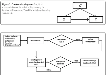
con-founders. In Figure  we provide a graphical representation of the dependencies between

the treatment, outcome and confounding variables. Theidentification of the confounders

Figure 1 Confounder diagram.Graphical representation of the relationships among the treatmentX, outcomeYand the set of confounding variablesC.

Figure 2 Description of the causal inference process in observational data using a quasi-experimental matching design.

An unbiased causality study requires that the assignment of units to treatments is in-dependent from the outcome conditional to the confounding variables. While in experi-mental studies this requirement is satisfied by randomly assigning units to treatments, in observational studies we could eliminate confounding bias by comparing units with

simi-lar values on their confounding variables but different treatment value (matching design).

Let us consider a binary treatmentX, a group oftreatedunitsUand a group ofcontrol

unitsVsuch asXu= ,∀u∈UandXv= ,∀v∈V. Let us also consider a set of confounding

variablesC. Ideally, each unitu∈Uwill be matched with a unitv∈VifCi

u=Cvi,∀Ci∈C. However, perfect matching is usually not feasible. Thus, treated units need to be matched

with themost similarcontrol units. Several methods have been proposed to create

bal-anced treated and control pairs []. After applying a matching method, it is necessary to check whether the treated and control groups are sufficiently balanced by estimating the standardized mean difference between the groups or by applying graphical methods such as quantile-quantile plots, cumulative distribution functions plots, etc. []. If sufficient balance has not been achieved, the matching method has to be revised.

Finally, if any confounding bias has been sufficiently eliminated, the treatment effect can

be estimated by comparing the effect variableYof the matched treated and control units.

Let us define asGthe set of paired treated and control units andNGthe number of pairs.

Then, the average treatment effect (ATE) can be estimated as follows:

ATE=

∀(u,v)∈GYu–Yv

NG

. ()

3 Dataset description

The StudentLife dataset contains a rich variety of information that was captured either through smartphone sensors or through pop-up questionnaires. In this study we use only GPS location traces, accelerometer data, a calendar with the deadlines for the modules that students attend during the term and students responses to questionnaires about their stress level. Students answer to these questionnaires one or more times per day.

We use the location traces of the users to create location clusters. GPS traces are pro-vided either through GPS or through WiFi or cellular networks. For each location cluster,

we assign one of the following labels:home,work/university,gym/sports-center,

socializa-tion venueandother. Labels are assigned automatically without the need for user inter-vention (a detailed description of the clustering and location labeling process is presented in Additional file ).

We use information extracted from both accelerometer data and location traces to infer whether participants had any exercise (either at the gym or outdoors). The StudentLife dataset does not contain raw accelerometer data. Instead it provides an activity classi-fication by continuously sampling and processing accelerometer data. The activities are classified to stationary, walking, running and unknown.

We also use the calendar with students’ deadlines, which is provided by the StudentLife

dataset, as an additional indicator of students workload. We define asDu_deadlinethe set of

all days that the studentuhas a deadline. We define a variableDu,d_{that represents how}

many deadlines are close to the daydfor a useruas follows:

Du,d=

⎧ ⎨ ⎩

j∈Du_deadline

j j–d, ifj–Tdays<d<j,

, otherwise. ()

Thus,Du,d _{will be equal to zero if there are no deadlines within the nextT}

days days,

whereTdaysis a constant threshold; otherwise,Du,dwill be inversely proportional to the

number of days remaining until the deadline. In our experiments we set theTdaysthreshold

equal to . We found that with this value the correlation between the stress level of the

participants and the variableDu,d_{is maximized.}

Finally, the StudentLife dataset includes responses of the participants to the Big Five Personality test []. The Big Five Personality Traits describe human personality using

five dimensions:openness,conscientiousness,extroversion,agreeableness, andneuroticism.

The personality traits of participants can be used to describe some baseline characteristics of the units and, for this reason, we include them in the study.

4 Causality analysis

We apply the causal inference framework described in the previous section in order to assess the causal impact of factors like exercising, socializing, working or spending time

at home on stress level.a

4.1 Variables

Initially, we define the variables that will be included in the study as follows:

 H_tu,d: denotes the total time in seconds that the useruspent at home during dayd

 Utu,d: denotes the total time in seconds that the useruspent at university during dayd

until timet;

 Ou_t,d: denotes the total time in seconds that the useruspent in any place apart from

his/her home or university during dayduntil timet;

 Eut,d: denotes the total time in seconds that the useruspent exercising during dayd

before timet(it is estimated using both location traces and accelerometer data);

 SCu_t,d: denotes the total time in seconds that the useruspent at any socialization or

entertainment venue during daydbefore timet;

 Sut,d: denotes the stress level of useruthat was reported on daydand timet. Stress

level is reported one or more times per day. Thus, in contrast with the above

mentioned variables,S_tu,dis not continuously measured;

 PSu,d_{: denotes the last stress level that was reported by useruduring the dayd– .}

This variable remains constant within a day;

 Du,d_{: represents the upcoming deadlines as described in Eq. ();}

 Eu_,Nu_,Au_,Cu_,Ou_{: these five variables denote the extroversion, neuroticism,}

agreeableness, conscientiousness and openness of userubased on his Big Five

Personality Traits score respectively.

4.2 Units

In this study, we examine the effects of five treatments, denoted by the variables Htui,d,

U_tu_i,d, Ou_ti,d, Eu_ti,d andSCu_ti,don the stress level of participants, which is described by the

variableSu_t,d. A unit of the study corresponds to a set of attributes derived by the variables

of the experiment. All the variables are sampled every  hours, thus there are maximum

six samples per day for each participant. LetT={ am,  am,  pm,  pm,  pm,  pm}

a set of sampling times andtitheith element ofT. Then, a unit corresponds to the set of

variablesPu_ti,d= (H_tu_i,d,U_tu_i,d,Ou_ti,d,Eu_ti,d,SCu_ti,d,Su_ti,d,PSu,d_,Du,d_{). Since the variableS}u,d

t is not

continuously measured, it is not feasible to sample it for timeti. Instead, we defineSuti,das

the average stress level of unituin daydbetween timetiandti+. Thus,Stui,dis estimated

as follows:

Su_ti,d=ES_tu,d, forti≤t≤ti+. ()

If there are no stress level reports during this time interval, then the unit that

corre-sponds to the set of variablesPu_ti,dwill be discarded.

4.3 Detection of confounding variables

time that students spend at home and university and their deadlines. Moreover, partici-pants choice to do an activity may exclude another activity from their schedule and it may also influence their stress level. For example, someone may choose to spend some time in a pub instead of following his/her normal workout schedule. The previous day stress level may also influence both next day’s activities and stress level. Finally, several studies have demonstrated that stress level fluctuations are affected by personality traits []. In general, more positive and extrovert people tend to be able to handle stress better than people with high neuroticism score. Moreover, personality characteristics may correlate with the daily schedule that people follow. For example, more extrovert people may spend less time at home and more time in social activities. In order to define the covariates of the study, we conduct a correlation analysis on the variables of interest. Since the relationship among

the variables may not be linear, we apply the Kendall rank correlation. Thep-values of the

Kendall correlation are presented in Table .

Based on these results, the time that students spend at home does not correlate with

their stress level. Thus, the variableH_tu_i,dwill not be included in the causality study. The

causal impact of each treatment variableUtui,d,O

u,d ti ,E

u,d ti andSC

u,d

ti on the effect variable

Suti,dwill be examined using all the variables that correlate with both the treatment and

ef-fect based on Table  as confounding variables. We consider a correlation to be significant

enough if thep-value is smaller than .. In Table , we present the confounding

vari-ables that will be used for each examined treatment. While the varivari-ablesOuti,dandSC

u,d ti

are strongly correlated, we do not includeSCuti,din the set of confounding variables when

the treatment is the variableOu_ti,d, since our goal is to study the impact of spending time

in any place (including socialization venues) apart from home and working environment.

Table 1 p-values of Kendall correlation under the null-hypothesis that the examined variables are independent

Su,d_ti Hu,d_ti U_tiu,d Ou,d_ti Eu,d_ti SCu,d_ti

Hu_ti,d 0.3557 0 6·10–128 7·10–182 0.0161 2.7·10–6

Uu_ti,d 0.004 6·10–128 _{0 2·10}–6 _{0.042 0.024}

Ou_ti,d 6·10–5 _7·10–182 _2·10–6 _{0 10}–7 ₁₀–13

Eu_ti,d 0.0081 0.0161 0.042 10–7 _{0 0.222}

SCu_ti,d 9·10–5 _2.7·10–6 _{0.024 10}–13 _{0.222 0}

PSu,d 2.7·10–59 _{0.967 0.0071 0.055 0.3897 0.046}

Du,d _{0.024 2.5·10}–6 _{0.0014 0.0018 0.002 0.0076}

Eu _1.69·10–11 _2.27·10–5 _{0.059 4.9·10}–4 _4.1·10–5 _0.0037

Nu 1.81·10–14 0.004 1.2·10–5 2.3·10–16 0.013 6·10–6

Au 0.007 0.21 0.15 0.047 0.006 0.002

Cu 0.057 0.078 0.01 0.47 0.352 0.214

Ou 0.604 0.006 0.005 2.1·10–5 4.7·10–4 0.95

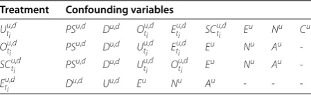
Table 2 Confounding variables for the different applied treatments

Treatment Confounding variables

Uu_ti,d PSu,d Du,d _Ou,d

ti Etiu,d SCtiu,d Eu Nu Cu

Ou_ti,d PSu,d Du,d _Uu,d

ti Etiu,d Eu Nu Au

-SCu_ti,d PSu,d Du,d _Uu,d

ti Outi,d Eu Nu Au

-4.4 Creation of treated and control groups

After defining the confounding variables of the study, we need to split the units into con-trol and treatment groups. We consider binary treatments by applying thresholds to the

examined treatment variables. Thus, for each of the four examined treatments (i.e.,Utui,d,

O_tu_i,d,E_tu_i,d,SCu_ti,d) the units are split as follows:  Utui,d: treatment units are all the units withU

u,d ti <E{U

u,d

ti }–α·E{U

u,d

ti }and control all

the units withU_tu_i,d≥E{U_tu_i,d}+α·E{U_tu_i,d}, for a constantα∈[, ). Thus, we consider to have a positive treatment value when the university sojourn time is relatively small;  Ou_ti,d: treatment units are all the units withO_tu_i,d>E{U_tu_i,d}+α·E{U_tu_i,d}and control all

the units withOuti,d≤E{U

u,d

ti }–α·E{U

u,d

ti }. Thus, we consider to have a positive

treatment value when the time spent in any non-work-related place outside home is relatively large;

 Etui,d: treatment units are all the units withE

u,d

ti > i.e. all the units that denote that a

useruhad some exercise at daydbefore timet. In the control group are units with

Euti,d= ;

 SCuti,d: similarly to the treatment variableE

u,d

ti , treatment units are units withSC

u,d ti >  and control units withSCuti,d= .

Thus, when the treatment variablesUtui,dandO

u,d

ti are considered, units are classified

as treated and untreated based on the time participants have spent at university or at any place apart from their home and university, respectively. However, in order to examine the impact of exercising and visiting socialization venues, the binary treatments are defined by considering only whether there was some exercising activity or a visit to a socialization place or not. We do not study the impact of these factors by considering also the duration of these events since the amount of the data is not sufficiently large.

Each of the examined treatment variables describes some user behavior or activity from

the start of the day to some timeti. Consequently, the comparison of two units with

dif-ferent sampling timestiis not valid. Thus, we create a group of pairs of treated and

con-trol unitsGti for each one of the  sampling timestisuch that each treated unitP

(u,d)

ti is

matched with a control unitP(tui,d)with similar values on its confounding variables. Then,

the average treatment effect is estimated as follows:

ATE=

ti

(P(_tiu,d),P_ti(u,d))∈G_ti(SP_ti(u,d)–SP_ti(u,d))

tiNGti

. ()

If there is no causal effect of the examined treatment on the stress level then the average

treatment effect should be zero. We use at-test in order to decide whether the observed

average treatment effect is statistically significant.

4.5 Balance check

In order to create balanced treated and control pairs of units we apply the Genetic Match-ing method []. Genetic MatchMatch-ing is a multivariate matchMatch-ing method that applies an evolutionary searching algorithm that estimates weights for each confounding variable in order to achieve an optimal covariates balance. In order to assess if the treated and control pairs are sufficiently balanced, we check the standardized mean difference for each

each confounding variablec∈C, the standardized mean difference is estimated as follows:

SMDc=

∀ti

∀(P(_tiu,d),P_ti(u,d))∈G_ti(cP(_tiu,d)–cP_ti(u,d))

∀tiNGti

σT=

c , ()

whereσ_cT=denotes the variance of the confounding variablecfor the treated units. The

remaining bias from a confounding variablecis considered to be insignificant ifSMDcis

smaller than . [].

5 Results

We conduct a causal inference study for each one of the four examined treatments that were discussed above. In each study, we use as confounding variables all the variables that are presented in Table . We report our findings collectively for the whole population. We also repeated these studies separately for participants with high and low extroversion and participants with high and low neuroticism scores in order to investigate whether some of the examined treatments have a different causal impact on these sub-populations. We decided to conduct additional studies separately for these sub-populations because neu-roticism and extroversion are strongly correlated with stress level according to Table .

Participants are classified ashighly extrovertsif their extroversion score is higher than the

average extroversion score; otherwise, they are classified as member of thelow

extrover-sionsub-population. Correspondingly, we define two sub-population of participants with

high neuroticism(i.e. participants with neuroticism score higher than the average) and

participants withlow neuroticismscores. In Figure  we present the distribution of the

neuroticism and extroversion scores of the participants.

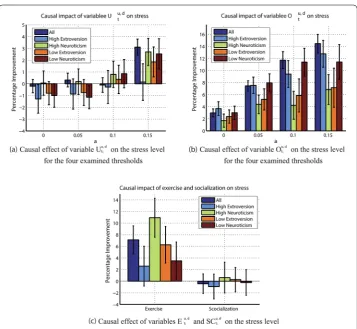
In Figure  we show the average treatment effect (ATE) normalized by the average stress level of the control units along with the % confidence intervals for each one of the four

examined treatment variables. For the treatment variablesU_tu_i,dandOu_ti,dwe present results

forαequal to , ., . and .. We do not present results for largerαvalues since the

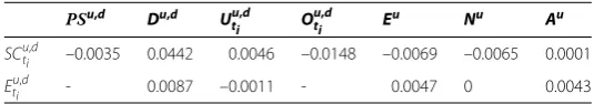
number of samples that are discarded is large and the remaining data are not sufficient for statistically significant conclusions. In Figure  and Table  we present the standardized difference, as described in Eq. (), for all the confounding variables that were used in each one of the causation studies. According to our results, the standardized difference between treated and control samples is smaller than . for all the confounding variables thus any confounding bias has been sufficiently minimized.

Figure 4 Treatment effect.Percentage improvement on the stress level of treated units compared to control units when each one of the examined treatments is applied. Percentage improvement is estimated as

ATE

E{S(_tiu,d)}×

100. Results are presented along with the 95% confidence interval.

Figure 5 Balance check.Standardized difference between treated and control samples for each

Table 3 Standardized difference between treated and control samples for each one of the confounding variables when the applied treatments correspond to the variablesSCu,d_t

i

andE_tu,d i

PSu,d Du,d _Uu,d ti O

u,d

ti Eu Nu Au

SCu_ti,d –0.0035 0.0442 0.0046 –0.0148 –0.0069 –0.0065 0.0001

Eu_ti,d - 0.0087 –0.0011 - 0.0047 0 0.0043

Our results indicate that the time that students spend at university has only a weak causal impact on the stress level when participants’ samples are split into treatment and control

groups using anαvalue equal to .. In detail, participants report .% (with confidence

interval±.%) lower stress level the days that their sojourn time at university is % lower

than the average university sojourn time of the whole population compared to days that the university sojourn time is % larger than usual. However, when the analysis is limited to people with high extroversion score, there is no statistically significant evidence that

the time that students spend at university has any causal effect on stress. When smallerα

values are considered, the causality score is close to zero for the examined set of students. Based on our results, the time that students spend in any place apart from their home and university has a significantly strong causal impact on their stress level. As depicted in

Figure (b), students have reported around % (with confidence interval±.%) lower

stress level the days that they spend more time outside than the average time compared

to days that they spend less time outside (i.e.,α= ), when the whole set of participants

is considered. Similar results are observed when the study is repeated separately for stu-dents with high and low extroversion and stustu-dents with high and low neuroticism scores (the observed difference is not statistically significant given the % confidence intervals

of the study). When the value ofα is increased, the causal impact of the examined

vari-able is stronger. Forα= ., the improvement on the stress level for students who spend

more time outside is .% (with confidence interval±.%) when the total population is

considered. The results are similar when the study is limited to students with high extro-version score and students with low neuroticism scores. However, the examined variable has a significantly lower impact on stress level when only students with high neuroticism score and students with low extroversion score are considered.

In Figure (c), we examine the impact of exercising or visiting socialization venues on

stress level. While the variableSCuti,dis strongly correlated with the stress level,

accord-ing to our results, there is no causal link between them. This indicates that, while people benefit from spending time outside home or working environment in general, there is no statistically significant benefit from visiting specific venues. Finally, exercising has positive effect on the stress level of the examined population. When we examine the four different sub-populations separately, we observe that exercising has a stronger positive effect on the stress level of participants with high neuroticism score while there is no statistically significant benefit for people with high extroversion score. The impact on people with low neuroticism score is also weak.

6 Discussion

as working, exercising and socializing, on stress level of  students using data captured by means of smartphone sensors. Our study does not consider the impact of social influence on stress level of individuals mainly because of dataset limitations (see endnote a). Our re-sults suggest that exercising and spending time outside home or university have a strongly positive causal effect on participants’ stress level. We have also demonstrated that the time participants stay at university has a positive causal impact on their stress level only when it is considerably lower than the average daily university sojourn time. However, this impact is not remarkable.

Moreover, we have observed that some of the examined factors have different impact on the stress level of students with high extroversion score and on students with high neu-roticism score. More specifically, more extrovert students benefit more from spending time outside home or university, while more neurotic students benefit more from exercis-ing.

Our study mainly relies on raw sensor data that can be easily captured with smartphones. We have demonstrated that information extracted by simply monitoring users’ location and activity (through accelerometer) can serve as an implicit indicator of several factors of interest such as their working and exercising schedule as well as their daily social in-teractions. Inferring this high-level information using raw sensor data instead of pop-up questionnaires has three main advantages: () it offers a more accurate representation of participants activities over time since data are collected continuously; () data are col-lected in an obtrusive way without requiring participants to provide any feedback; this minimizes the risk that some users will quit the study because they are dissatisfied be-cause of the amount of feedback that they need to provide; () data gathered through pop-up questionnaires may not be objective since participants may provide either inten-tionally or uninteninten-tionally false responses. On the other hand, inferences based on sensor data could also be inaccurate either due to noisy sensor measurements or due to the fact that the variable of interest is inferred by the sensed data rather than directly measured. For example, in our case we assume that a visit to a sports center implies that the user had some exercise. However, the user may have visited this place to attend a sport event or just to meet friends. Assessing the degree of uncertainty that information inference from sensor measurements involves and incorporating this uncertainty into the causation study represents an interesting research area for further investigation.

This study involves a limited number of participants who do not constitute a repre-sentative sample of the population; therefore extrapolating general conclusions about the causal impact of the examined factors on stress level is not feasible. However, the purpose of this article is to demonstrate the potential of using smartphones for conducting large-scale studies related to human behavior, rather than present a thorough investigation on factors influencing the stress level of the participants.

Additional material

Additional file 1: Supplementary material(pdf )

Competing interests

The authors declare that they have no competing interests.

Authors’ contributions

FT and MM designed the study. FT analyzed the data and prepared the figures. FT and MM wrote the manuscript.

Author details

1_{School of Computer Science, University of Birmingham, Edgbaston, Birmingham, B15 2TT, United Kingdom.} 2_{Department of Geography, University College London, Gower Street, London, WC1E 6BT, United Kingdom.}

Acknowledgements

This work was supported through the EPSRC Grants “Trajectories of Depression: Investigating the Correlation between Human Mobility Patterns and Mental Health Problems by means of Smartphones” (EP/L006340/1) and “MACACO: Mobile context-Adaptive CAching for Content-Centric networking” (EP/L018829/1).

Endnote

a _{There are some studies which provide evidence that mood of individuals is influenced by the mood of their peers}

(see for example [27, 29]). However, the dataset limitations do not allow us to investigate whether the stress experienced by a participant could influence his/her social circle. In order to examine this aspect, we create a friendship network based on the phone calls/SMSes of the users. However, the resulting friendship network is composed of only 19 students out of 48 (i.e., there were only 19 students with at least one friendship link to another student). Moreover, all the users are not active during all the days of the study (e.g., some users do not report their stress level every day). In order to study the impact of friends’ stress, we need to consider only samples for which we have information for both the stress level of the student taken into consideration and the stress level of his/her friends. This reduces the size of our dataset by 73%. The sample is not sufficient to derive statistically significant results. For this reason, the impact of the social network of individuals is not considered in this study.

Received: 5 May 2015 Accepted: 27 November 2015

References

1. Miluzzo E et al (2008) Sensing meets mobile social networks: the design, implementation and evaluation of the CenceMe application. In: Proceedings of SenSys’08. ACM, New York, pp 337-350

2. Ravi N, Dandekar N, Mysore P, Littman ML (2005) Activity recognition from accelerometer data. In: Proceedings of AAAI’05, vol 3, pp 1541-1546

3. Lu H, Rabbi M, Chittaranjan GT, Frauendorfer D, Mast MS, Campbell AT, Gatica-Perez D, Choudhury T (2012) StressSense: detecting stress in unconstrained acoustic environments using smartphones. In: Proceedings of UbiComp’12. ACM, New York, pp 351-360

4. Rachuri KK, Musolesi M, Mascolo C, Rentfrow PJ, Longworth C, Aucinas A (2010) Emotionsense: a mobile phones based adaptive platform for experimental social psychology research. In: Proceedings of UbiComp’10. ACM, New York, pp 281-290

5. Ma Y, Xu B, Bai Y, Sun G, Zhu R (2012) Daily mood assessment based on mobile phone sensing. In: Proceedings of BNS’12. IEEE, Los Alamitos, pp 142-147

6. Bauer G, Lukowicz P (2012) Can smartphones detect stress-related changes in the behaviour of individuals? In: Proceedings of PerCom Workshops’12. IEEE, Los Alamitos, pp 423-426

7. Bogomolov A, Lepri B, Pianesi F (2013) Happiness recognition from mobile phone data. In: Proceedings of SocialCom’13. IEEE, Los Alamitos, pp 790-795

8. Bogomolov A, Lepri B, Ferron M, Pianesi F, Pentland AS (2014) Daily stress recognition from mobile phone data, weather conditions and individual traits. In: Proceedings of Multimedia’14. ACM, New York, pp 477-486 9. Canzian L, Musolesi M (2015) Trajectories of depression: unobtrusive monitoring of depressive states by means of

smartphone mobility traces analysis. In: Proceedings of UbiComp’15. ACM, New York

10. Asur S, Huberman BA (2010) Predicting the future with social media. In: Proceedings of the 2010 IEEE/WIC/ACM international conference on web intelligence and intelligent agent technology (WI-IAT), vol 1. IEEE, Los Alamitos, pp 492-499

11. Tumasjan A, Sprenger TO, Sandner PG, Welpe IM (2010) Predicting elections with Twitter: what 140 characters reveal about political sentiment. In: Proceedings of the fourth international AAAI conference on weblogs and social media, pp 178-185

12. Bollen J, Mao H, Zeng X (2011) Twitter mood predicts the stock market. J Comput Sci 2(1):1-8

13. Cha M, Haddadi H, Benevenuto F, Gummadi PK (2010) Measuring user influence in Twitter: the million follower fallacy. In: Proceedings of the fourth international AAAI conference on weblogs and social media, pp 10-17 14. Anger I, Kittl C (2011) Measuring influence on Twitter. In: Proceedings of KDD’11. ACM, New York, p 31 15. Bond RM, Fariss CJ, Jones JJ, Kramer ADI, Marlow C, Settle JE, Fowler JH (2012) A 61-million-person experiment in

social influence and political mobilization. Nature 489(7415):295-298

16. Muchnik L, Aral S, Taylor SJ (2013) Social influence bias: a randomized experiment. Science 341(6146):647-651 17. Onnela J-P, Saramäki J, Hyvönen J, Szabó G, Lazer D, Kaski K, Kertész J, Barabási A-L (2007) Structure and tie strengths

18. Colizza V, Barrat A, Barthelemy M, Vespignani A (2006) Prediction and predictability of global epidemics: the role of the airline transportation network. Proc Natl Acad Sci USA 103:2015

19. Marsch LA (2012) Leveraging technology to enhance addiction treatment and recovery. J Addict Dis 31(3):313-318 20. Pejovic V, Musolesi M (2014) Anticipatory mobile computing for behaviour change interventions. In: Proceedings of

MCSS’14. ACM, New York, pp 1025-1034

21. Moturu ST, Khayal I, Aharony N, Pan W, Pentland AS (2011) Using social sensing to understand the links between sleep, mood, and sociability. In: Proceedings of SocialCom’11. IEEE, Los Alamitos, pp 208-214

22. Madan A, Moturu ST, Lazer D, Pentland AS (2010) Social sensing: obesity, unhealthy eating and exercise in face-to-face networks. In: Proceedings of wireless health 2010. ACM, New York, pp 104-110

23. Mouchart M, Russo F, Wunsch G (2009) Structural modelling, exogeneity, and causality. In: Causal analysis in population studies. Springer, Berlin, pp 59-82

24. Spirtes P, Glymour CN, Scheines R (2000) Causation, prediction, and search. MIT Press, Cambridge

25. Shadish WR, Cook TD, Campbell DT (2002) Experimental and quasi-experimental designs for generalized causal inference. Wadsworth Cengage Learning, Boston

26. Rosenquist JN, Murabito J, Fowler JH, Christakis NA (2010) The spread of alcohol consumption behavior in a large social network. Ann Intern Med 152(7):426-433

27. Fowler JH, Christakis NA et al (2008) Dynamic spread of happiness in a large social network: longitudinal analysis over 20 years in the Framingham Heart Study. Br Med J 337:2338

28. Cacioppo JT, Fowler JH, Christakis NA (2009) Alone in the crowd: the structure and spread of loneliness in a large social network. J Pers Soc Pychol 97(6):977

29. Rosenquist JN, Fowler JH, Christakis NA (2011) Social network determinants of depression. Mol Psychiatry 16(3):273-281

30. Christakis NA, Fowler JH (2013) Social contagion theory: examining dynamic social networks and human behavior. Stat Med 32(4):556-577

31. Wang R et al (2014) StudentLife: assessing mental health, academic performance and behavioral trends of college students using smartphones. In: Proceedings of UbiComp’14. ACM, New York, pp 3-14

32. Holland PW (1986) Statistics and causal inference. J Am Stat Assoc 81(396):945-960

33. Stuart EA (2010) Matching methods for causal inference: a review and a look forward. Stat Sci 25(1):1 34. Austin PC (2011) An introduction to propensity score methods for reducing the effects of confounding in

observational studies. Multivar Behav Res 46(3):399-424

35. Bolger N, Schilling EA (1991) Personality and the problems of everyday life: the role of neuroticism in exposure and reactivity to daily stressors. J Pers 59(3):355-386