R E S E A R C H
Open Access
Analyzing the availability and
performance of an e-health system integrated
with edge, fog and cloud infrastructures
Guto Leoni Santos
1*, Patricia Takako Endo
2,3, Matheus Felipe Ferreira da Silva Lisboa Tigre
2,
Leylane Graziele Ferreira da Silva
1, Djamel Sadok
1, Judith Kelner
1and Theo Lynn
3Abstract
The Internet of Things has the potential of transforming health systems through the collection and analysis of patient physiological data via wearable devices and sensor networks. Such systems can offer assisted living services in real-time and offer a range of multimedia-based health services. However, service downtime, particularly in the case of emergencies, can lead to adverse outcomes and in the worst case, death. In this paper, we propose an e-health monitoring architecture based on sensors that relies on cloud and fog infrastructures to handle and store patient data. Furthermore, we propose stochastic models to analyze availability and performance of such systems including models to understand how failures across the Cloud-to-Thing continuum impact on e-health system availability and to identify potential bottlenecks. To feed our models with real data, we design and build a prototype and execute performance experiments. Our results identify that the sensors and fog devices are the components that have the most significant impact on the availability of the e-health monitoring system, as a whole, in the scenarios analyzed. Our findings suggest that in order to identify the best architecture to host the e-health monitoring system, there is a trade-off between performance and delays that must be resolved.
Keywords: Cloud computing, Data center failure, Emergency call service, Availability, Edge computing, Fog computing; e-health
Introduction
The rapid emergence, ubiquity, and convergence of social media, mobility, cloud computing, big data and data ana-lytics, and the Internet of Things (IoT) are transforming how society operates and interacts with each other. Unsur-prisingly, the health sector is a major focus of IoT research by both academia and industry due to its potential to reduce costs, increase patient quality of life, and enrich the patient experience [1]. Authors in [2] suggest that the underlying concept of IoT is the pervasive presence of a variety of connected things that can interact with each other and cooperate with their neighboring devices (things) to reach common goals. Things can be sensors,
*Correspondence:[email protected]
1Universidade Federal de Pernambuco (UFPE), Grupo de Pesquisa em Redes de Computadores e Telecomunicações (GPRT), Recife, Pernambuco, Brazil Full list of author information is available at the end of the article
actuators, smart phones, computers, home/work appli-ances, cars, and any other object that can be connected, monitored and/or actuated [3]. IoT applications have the potential of significantly impacting the everyday-life of users, and are visible in many aspects of modern soci-ety including smart cities, smart factories, traffic control, assisted living, e-health etc.
IoT is not without its challenges. The relatively small size and heterogeneity of connected edge devices typically results in limited storage and processing capacity, and consequential issues regarding reliability, performance, and security [4]. These limitations are exacerbated when one considers that IoT applications typically require sig-nificant data storage and processing as well as high-speed broadband networks to enable real-time decision making [5]. For instance, in the case of e-health monitoring sys-tems, while the data generated by sensors could be used in diagnostic scenarios ranging from spine injuries to heart disease to cancer, medical image analysis often requires
high performance processing and storage resources that are not available from edge devices.
Some of these IoT issues can be mitigated by integrat-ing fog and cloud computintegrat-ing (hereafter referred to as as IoT-to-cloud (I2C) system, crossing from edge devices, fog devices and cloud infrastructure). Cloud comput-ing is now a relatively mature technology and offers IoT use cases improved processing and storage capabil-ities, scalability, and availability. Fog computing, a rela-tively new paradigm recognizes the limitations of existing telecommunications networks and connected devices. It extends the cloud paradigm to the edge of the net-work thereby enabling and supporting vertically-isolated, latency-sensitive applications [6, 7]. Many applications require both fog localization and cloud globalization par-ticularly for data analytics and big data use cases. Fog is particularly well suited to real-time streaming analytics as opposed to historical, big data batch analytics that is normally carried out in a data center [8].
Despite the advantages that cloud and fog comput-ing brcomput-ing to IoT applications, they also introduce an added layer of management complexity. While improving availability, they introduce new points of failure beyond the discreet IoT device i.e. failures in fog devices and cloud infrastructure components, or as a whole. Avail-ability is critical in many e-health applications partic-ularly those that are actively monitoring patient health and informing decisions by the patient or their health professionals. Any downtime in critical e-health moni-toring systems or lost data, including loss of data to the patient, results in any subsequent medical analysis being compromised, putting the patients well-being and life at risk.
Traditional e-health monitoring systems adopt a con-tinuous monitoring strategy. According to [9],“such long-term monitoring consumes storage, uses energy for multiple sensors and sinks, increases computational costs required to analyze data, and increases network usage leading to transmission failures”. As a result, in addition to availabil-ity analysis, the system performance requires additional analysis to identify system bottlenecks and propose solu-tions to mitigate or resolve them.
However, results from pure availability analysis tend to be simplistic since models consider that a sys-tem has only two states (functioning or failed). On
the other hand, “pure performance analysis of a
sys-tem tends to be optimistic since it ignores the fail-ure/repair behavior of the system” [10]. To address these issues, we combine availability and performance mod-eling and analysis to present a more robust evalua-tion of the target system, in this case an e-health monitoring system.
Some existing works from the literature, such as [11–14], have proposed models for e-health systems in
the IoT context. However, none of them have consid-ered the integrated scenario relying on edge, fog, and cloud infrastructures. Similarly, both availability and per-formance models are not tested. Only [14] has considered a real testbed to perform experiments however in this case, they did not present e-health use cases. As such, this paper extends the state of the art through the following contributions:
• we proposestochastic availability modelsto understand how failures in edge devices, fog devices, and/or cloud infrastructure impacts on e-health monitoringsystem availability. These models will also be used to performsensitivity analysisto understand which components have a significant impact on the I2C-based e-health monitoring system availability;
• we implement aprototypeto conduct performance evaluations in order to feed the stochastic models with real data. This prototype is composed of two different configurations of fog devices, two different network connections to access the cloud instance, and four different geo-locations of cloud instance in order to characterize the heterogeneity of I2C-based systems; and
• we proposestochastic performance models
integrated with the availability models, and real data outputted from the prototype in order to understand how different capacity of fog devices and also different geo-location of cloud instances impact on performance metrics, such as throughput and service time.
The remainder of this paper is organized as follows. Section3describes related works. In Section3, key con-cepts used in the study are presented. This is followed by our approach to modelling the e-health monitoring sys-tem in Section3. We then present our results in Section3.
The paper concludes in Section3with a summary of our
work and avenues for further research.
Related work
Fig. 1IoT system integrated with cloud and fog computing applied in a smart city scenario
account both service requirements and resource offerings in a fog-to-cloud scenario including parameters such as energy consumption balance and delay between the fog and cloud.
While these works propose models and evaluate I2C integration, they explore different domains with differ-ent levels of criticality. E-health monitoring systems, the focus of our study, has specific constraints not dealt with in the aforementioned works including the load gener-ated by the sensors. Authors in [11] propose a model to represent and evaluate the security of information flow in IoT systems integrated with cloud, using a medical application as an example. They analyzed how service provider availability affects the security of the informa-tion flow. Similarly, the authors in [11] use a medical application as a case study for their proposed model ana-lyzing the security of the information flow in IoT systems integrated with cloud infrastructures. In [12], the authors propose a framework that enables multiple applications
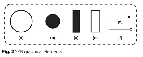
Fig. 2SPN graphical elements
to share IoT computational devices for health
monitor-ing. The use case scenario in [13] is a wearable IoT
architecture for health care systems. In [14], the authors propose stochastic models to represent a health service relying on mobile cloud computing infrastructure (i.e. cloud infrastructure, wireless communication and mobile device). Experiments were conducted considering scenar-ios with different wireless communication channels (Wi-Fi and 4G), different battery discharge rates, and different timeouts.
Our work differs from these works on e-health applica-tions because we consider an e-health I2C-based system that relies on edge, fog and cloud infrastructures. Based on this novel and emerging scenario, we propose stochastic models to evaluate the availability and performance of this system in three different scenarios. We are also conduct a sensitivity analysis to understand how different values of MTTF and MTTR impact on the availability of the system as a whole. Furthermore, we perform experiments using a prototype in order to obtain real data to use as an input to our stochastic models to give more realistic results and associated discussion.
Background
Fig. 3An e-health monitoring system architecture
Cloud, edge and fog computing
NIST defines cloud computing as “... a model for enabling ubiquitous, convenient, on-demand network access to a shared pool of configurable computing resources (e.g., net-works, servers, storage, applications, and services) that can be rapidly provisioned and released with mini-mal management effort or service provider interaction” [8]. The opportunities presented by the cloud comput-ing paradigm for IT efficiencies and business agility enabled by scalability, rapid deployment, and paralleli-sation are very attractive to enterprises of all sizes and sectors (Kim, 2009).
Cloud computing and IoT can be viewed as two comple-mentary technologies. The Cloud can compensate for the technological constraints of IoT devices, namely process-ing, storage and energy limitations, by offering a scalable, cost-effective solution for IoT use cases. Similarly, IoT extends the utility and value of the cloud out in to the real world where enterprises and end users interact with a wide variety of industrial and consumer settings [4]. Thus creating new economic value for both the public and private sector driven through increased asset utilization and employee productivity, improved supply chain and logistics, optimized customer experience, and accelerated innovation [17,18].
With the proliferation of connected devices and asso-ciated IoT applications, massive volumes of data are being generated at the edges of networks. For a variety
of reasons including intermittent connectivity and local quality of service (QoS) expectations, in many instances data is processed locally [19]. This scenario where compu-tation happens at the smart end device at the edge of the network, and the related limitations associated with com-putation at the extreme network periphery, is increasingly referred to as edge computing [20]. According to NIST [21], “edge is the network layer encompassing the smart end devices and their users to provide, for example, local computing capability on a sensor, metering or some other devices that are network-accessible”.
Fig. 4E-health monitoring system scenarios
and traditional cloud data centers [7, 22]. Thus, fog devices are situated closer to the edge devices and can provide limited computational power for a lighter pro-cessing of the data collected by the edge devices, as illustrated in Fig.1.
Cloud and fog infrastructures, when integrated, can provide virtually unlimited computational capacity for IoT applications however the QoS and the availability of the cloud infrastructure and fog devices becomes critical dependencies in the overall system. The availability of IoT applications can be impacted by several factors includ-ing IoT and fog device failures, as well as issues relatinclud-ing
to the cloud infrastructure that impact QoS and avail-ability. The impact of these failures can be exacerbated by the complexity, interdependencies and interconnectiv-ity of the overall integrated system. As discussed earlier, there are many IoT e-health use cases where unavailabil-ity of service (even if only for a few seconds) can result in negative patient outcomes ranging from inconvenience to misdiagnosis, and in extreme cases, death. To understand the impact of e-health monitoring system unavailability resulting from fog and cloud failures, we model this sce-nario using a combination of Stochastic Petri Nets (SPN) and Reliability Block Diagrams (RBD).
Table 1Guard functions
Transition Guard Function
Fail_System_1 (#Sensors_ON=0)OR(#Microcontroller_ON=0)OR (#Fog_ON=0)OR(#Cloud_ON=0)
Repair_System_1 (#Sensors_ON=1)AND(#Microcontroller_ON=1)AND (#Fog_ON=1)AND(#Cloud_ON=1)
Fail_System_2 (#Sensors_ON=0)OR(#Microcontroller_ON=0)OR (#Cloud_ON=0)
Repair_System_2 (#Sensors_ON=1)AND(#Microcontroller_ON=1)AND (#Cloud_ON=1)
Fail_System_3 (#Sensors_ON=0)OR(#Microcontroller_ON=0)OR (#Fog_ON=0)
Repair_System_3 (#Sensors_ON=1)AND(#Microcontroller_ON=1)AND (#Fog_ON=1)
Reliability block diagrams
RBD is an instrument that allows relationships to be created amongst the components of a system and is fre-quently used to perform analyses, such as availability, maintainability, reliability allocation and design improve-ment decisions based on them [24].
According to [25], an RBD aims to represent the
behavior of a system using a graphical structure com-posed of connected blocks. There are two basic types of configuration: serial and parallel. The former is composed of serial nodes to represent the components of the sys-tem. It is similar to logical AND gates i.e. if at least one component fails, the whole system also fails. The latter is composed of parallel nodes that are similar to logical OR gates i.e the system is considered in fault only if all components fail [26,27].
RBDs are commonly used due their simplicity, but they can not be used to represent systems with more complex behavior [28]. Thus, Stochastic Petri Nets (SPNs) can be used to overcome this deficiency of RBDs.
Stochastic petri nets
A Petri Net is defined as a directed bipartite graph that can be used in modelling and describing informa-tion systems; it contains components in its structure such as sets of places and transitions [29, 30]. Petri Nets are called stochastic when each one of the its transitions are associated with a random firing delay that follows a stochastic process (normally following an exponential distribution) [31].
The main components of an SPN are shown in Fig.2.
Places (a) are represented as white circles, while tokens (b) are represented by black circles. Tokens are attached to places, and a set of tokens associated in places
can represents a state of system modeled. Transitions are represented by bars and can be enable according preconditions. Transitions can also be divided in to two types: (c) immediate (activated by distribution probabil-ity) and (d) timed (activated instantly). Arcs (e) (f ) connect places and transitions together and may have weight [32].
Sensitivity analysis
In [33], sensitivity analysis is defined as a paradigm that studies how the variation in output is associated to the variation of different inputs of a numerical model. Sensi-tivity analysis commonly presents some questions that are associated with it, such as “Is there any factor whose vari-ability has a negligible effect on the output?” and “What input factors cause the largest variation in the output?”. Sensitivity analysis targets different points according the application in focus and it can be used to explore several features of a model and an application. The objectives can cover regions of sensitivity, factor importance and func-tion, factor interdependence, assessment of the similarity, factor and model reduction, and uncertainty
apportion-ment [34]. The most common method of conducting
sensitivity analysis is to repeat the experiment by varying only one parameter of the system, while the others remain fixed [35] and doing the same for all components of the system. At the end of the experiment, a sensitivity ranking is generated based on the analysis of the outputs obtained from each observation.
Modeling an e-health monitoring system
Handling massive amounts of data can also impair the sys-tem in triggering relevant and timely decision making and actuation. In order to enhance the reliability of data trans-mission and the availability of highly relevant contextual
Fig. 7Cloud server model
information, there is a need to define efficient data sum-marizing and filtering mechanisms that can be applied with a conditional scheme [9].
E-health monitoring system
The popularization of smart end devices, tied to the advances in information and network technologies in recent years, have made possible the development of cheaper and more affordable medical systems. IoT has played an important role in the evolution of these systems, providing (low cost) sensors to monitor many aspects of patient life [36].
As described previously, edge devices can use cloud computing to improve the availability and performance of medical applications. For instance, Sierra wireless1
enables the connection between IoT devices and cloud computing infrastructure to collect and analyze real time data from hospitals and home health monitoring devices [36]. As an e-health monitoring system monitors a patient continuously, it collects vast amounts of data that needs to be analyzed in relative real-time without interruption. Significant delays in receipt of data can compromise the efficacy of an e-health application and impact the patient’s
well-being and health. In this case, according to [8], fog is positioned to play a significant role in the ingestion and processing of the data close to the source as it is being produced.
In this work, we propose an architecture to represent the behavior of an e-health monitoring system that relies on sensors, fog devices (such as Raspberry Pi2) and cloud infrastructure (public or private cloud services) to process and store patients vital signs data. Figure 3 presents our proposed architecture. We assume that patients have sensors (such as blood sugar measurement, heartbeat monitoring, and epileptic seizure detection) that collect the relevant physiological data and these sensors are cou-pled to a microcontroller (such as Arduino3). We also
assume that we have two different applications that
con-sume collected data: (a) a fog application, and (b) a
cloud application. We refer to these applications as web applications.
The fog application can check the normality of the data and, in the case of an anomaly, the application may instigate an action e.g. a call to an emergency service. Physiological data may be sent to the cloud application for further processing e.g. to train a machine learning
Fig. 9Performance model of e-health monitoring system
algorithm to examine a patient’s condition over time and to compare one patient against a larger population to help doctors to provide better treatment4.
Given this architecture, we consider three different availability scenarios (see Fig. 4) in which our e-health monitoring system is implemented:
• Scenario 1: The e-health monitoring system availability depends on all components of the system i.e. a failure in any of them will result in a system failure. This scenario does not present redundancy and the two applications are complementary i.e. when one of them fails, the system becomes unavailable. Data is sent to fog devices to perform some pre-processing that does not require large computational capacity. Later, the data is sent from the fog device to
Table 2Guard functions of performance model
Transition Guard function
ET1 #Sensor_up>0
ET2 #Cloud_up>0
ET3 #Cloud_up>0
ET4 #Fog_up>0
IT1 (#scenario=1)AND(#Microcontroller_ON>0)AND(#Fog_ON>0)
IT2 (#scenario=2)AND(#Microcontroller_ON>0)
IT3 (#scenario=3)AND(#Microcontroller_ON>0)
a cloud server to complete the processing and stored. A similar scenario is presented in [37];
• Scenario 2: The e-health monitoring system relies only on the cloud application and infrastructure to send patient vital signs data. As such, the system availability estimation does not take in account the fog application and fog device; and
• Scenario 3: This scenario is similar to scenario 2 but here the system relies only on the fog application and infrastructure to receive the patient data; the e-health monitoring system availability estimation does not consider the cloud application and cloud
infrastructure.
Stochastic models
We use the Mercury tool5to model the e-health monitor-ing system and evaluate its availability and performance.
Availability models
Figure 5 shows our SPN model representing the whole
Table 3Equations for performance metrics
Scenario Metric Equation (Mercury tool sintaxe)
1 Throughput P{(#1_Cloud_Requests>0)AND(#Cloud_ON>0)}*(1/ST_Fog_Cloud)
Service time E{#1_Cloud_Requests}/(P{#1_Cloud_Requests>0}*(1/ST_Fog_Cloud))
2 Throughput P{(#2_Cloud_Requests>0)AND(#Cloud_ON>0)}*(1/ST_Cloud)
Service time E{#2_Cloud_Requests}/(P{#2_Cloud_Requests>0}*(1/ST_Cloud))
3 Throughput P{(#3_Fog_Requests>0))AND(#Fog_ON>0)}*(1/ST_Fog)
Service time E{#3_Fog_Requests}/(P{#3_Fog_Requests>0}*(1/Fog_Cloud))
By way of illustration, in the cloud building block,
the placeCloud_ON represents that the cloud provider
is running, and the place Cloud_OFF that it has failed
or unavailable. The transitionCloud_Failrepresents the cloud failure event (mean time to failure (MTTF) value),
while Cloud_Repair represents the time to repair the
cloud infrastructure (mean time to repair (MTTR) value). In this work, we consider that all failure and repair times are exponentially distributed [38, 39]. The other three components (sensors, microcontroller, and fog) follow the same logic.
Moreover, there are another three building blocks with immediate transitions (in the top of the figure) that repre-sent the system status in different scenarios. From left to right, those building blocks represent scenario 1, 2 and 3 respectively (described in Section3). Each scenario has a building block composed of ON and DOWN places and two immediate transitions. These places have the same semantic meaning as the previous ones, as well as the tran-sitions. The difference is that each transition is activated through a guard function instead of MTTF or MTTR values. These functions are presented in Table1.
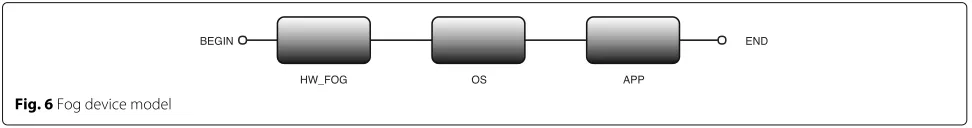
To provide more details about the fog device and cloud server that host an application, we modeled them as an RBD. To represent the fog device (Fig.6), we consider it is composed of hardware (HW), an operating system (OS), and the application (APP) that consumes the vital signs data from the patients. If any of these components fail, we consider that the fog device is unavailable and then the RBD is in series.
The cloud server (Fig. 7) is composed of hardware
(HW), an operating system (OS), a virtual machine (VM), and an application (APP) that will process the patients data to improve their treatment. We also consider that the failure of any component entails the cloud unavailability (RBD in series too).
The availability of each of the three scenarios is the probability of having a token in the place that represents the state ON of the respective building block (see Fig.5). To model the availability metric in our SPN, we utilize the following expression:
P{scenariox_ON}>0 (1) where xis the number of the scenario (from 1 to 3), as described previously.
Performance model
In this work, we consider a selection of performance met-rics based on [40]. To represent the clients requesting service, we consider a queuing systemM/M/1/K, mean-ing that the arrival process is a Poisson process with rate λ(M), the service time is independent and exponentially distributed with parameter μ (M), there is only a sin-gle server to process the requests (1), and the capacity of the system is limited (K). This queue configuration allows the evaluation of relevant aspects of the system, such as the impact of different arrival times and different queue capacities [41]; it is commonly used to represent cloud requests ([42–46]).
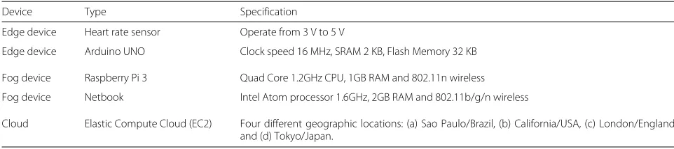
Table 4Prototype infrastructure components
Device Type Specification
Edge device Heart rate sensor Operate from 3 V to 5 V
Edge device Arduino UNO Clock speed 16 MHz, SRAM 2 KB, Flash Memory 32 KB
Fog device Raspberry Pi 3 Quad Core 1.2GHz CPU, 1GB RAM and 802.11n wireless
Fog device Netbook Intel Atom processor 1.6GHz, 2GB RAM and 802.11b/g/n wireless
Table 5Component configurations of scenario 1
Scenario Configuration Edge device Edge device Fog device Fog device network Cloud location
1 1 Heart rate sensor Arduino UNO Raspberry Pi 3 Ethernet Sao Paulo/Brazil
2 Heart rate sensor Arduino UNO Raspberry Pi 3 Ethernet California/USA
3 Heart rate sensor Arduino UNO Raspberry Pi 3 Ethernet London/England
4 Heart rate sensor Arduino UNO Raspberry Pi 3 Ethernet Tokyo/Japan
5 Heart rate sensor Arduino UNO Raspberry Pi 3 IEEE 802.11 Sao Paulo/Brazil
6 Heart rate sensor Arduino UNO Raspberry Pi 3 IEEE 802.11 California/USA
7 Heart rate sensor Arduino UNO Raspberry Pi 3 IEEE 802.11 London/England
8 Heart rate sensor Arduino UNO Raspberry Pi 3 IEEE 802.11 Tokyo/Japan
9 Heart rate sensor Arduino UNO Netbook Ethernet Sao Paulo/Brazil
10 Heart rate sensor Arduino UNO Netbook Ethernet California/USA
11 Heart rate sensor Arduino UNO Netbook Ethernet London/England
12 Heart rate sensor Arduino UNO Netbook Ethernet Tokyo/Japan
13 Heart rate sensor Arduino UNO Netbook IEEE 802.11 Sao Paulo/Brazil
14 Heart rate sensor Arduino UNO Netbook IEEE 802.11 California/USA
15 Heart rate sensor Arduino UNO Netbook IEEE 802.11 London/England
16 Heart rate sensor Arduino UNO Netbook IEEE 802.11 Tokyo/Japan
In order to illustrate how these performance metrics were modeled using an SPN approach, consider the
sim-ple queue model shown in Fig. 8. The transition T1
represents the arrival of clients while transitionT2 repre-sents the service time. We consider that both arrival time (AT) and service time (ST) are exponentially distributed [47,48]. The placeP1 represents requests that are in ser-vice. The placeP2 represents when the system resource (e.g. a web server) is running, whileP3 represents when a resource is in failure. TransitionsT_failureandT_repair
represent the failure and the repair of the resource, respec-tively.T2 only fires when there is a token in placeP2 i.e. when the resource is running and this behavior is assured by guard function #P2 > 0. The place P4 represents
the total capacity K that the system can withstand. In
other words, it is the number of requests can be queued in system.
In this work, we consider the following performance metrics6:
• Throughput (TP): can be defined as the rate requests can be serviced by the system. Generally, the
TP of a system increases as the load on the system increases. However, after a certain load level, the TP stops increasing, and, in most cases, even starts decreasing. In our system, the TP represents the number of requests the web applications (fog or cloud applications) can process. Taking into account the queue presented in Fig.8, TP can be calculated as the probability of having tokens in placeP1(requests in queue) and in placeP2(system working)
multiplied by the service rate:
TP=P{(#P1>0)AND(#P2>0)} ×(1/ST) (2)
• Service Time (ST): is, in a simplified way, the interval between a user’s request and the system response. In our system, we can define the interval between the HTTP request from the microcontroller and the response time of the web application (hosted either in the fog or cloud). Service time can be
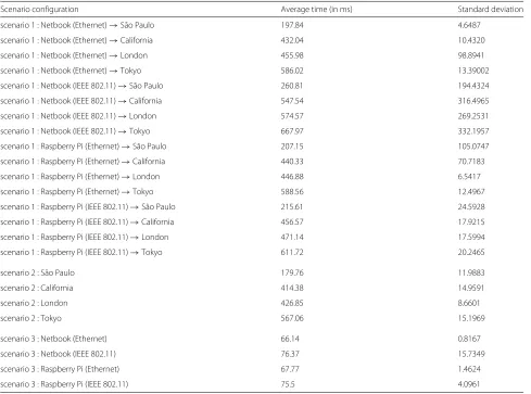
Table 6Results from prototype experiments
Scenario configuration Average time (in ms) Standard deviation
scenario 1 : Netbook (Ethernet)→São Paulo 197.84 4.6487
scenario 1 : Netbook (Ethernet)→California 432.04 10.4320
scenario 1 : Netbook (Ethernet)→London 455.98 98.8941
scenario 1 : Netbook (Ethernet)→Tokyo 586.02 13.39002
scenario 1 : Netbook (IEEE 802.11)→São Paulo 260.81 194.4324
scenario 1 : Netbook (IEEE 802.11)→California 547.54 316.4965
scenario 1 : Netbook (IEEE 802.11)→London 574.57 269.2531
scenario 1 : Netbook (IEEE 802.11)→Tokyo 667.97 332.1957
scenario 1 : Raspberry Pi (Ethernet)→São Paulo 207.15 105.0747
scenario 1 : Raspberry Pi (Ethernet)→California 440.33 70.7183
scenario 1 : Raspberry Pi (Ethernet)→London 446.88 6.5417
scenario 1 : Raspberry Pi (Ethernet)→Tokyo 588.56 12.4967
scenario 1 : Raspberry Pi (IEEE 802.11)→São Paulo 215.61 24.5928
scenario 1 : Raspberry Pi (IEEE 802.11)→California 456.57 17.9215
scenario 1 : Raspberry Pi (IEEE 802.11)→London 471.14 17.5994
scenario 1 : Raspberry Pi (IEEE 802.11)→Tokyo 611.72 20.2465
scenario 2 : São Paulo 179.76 11.9883
scenario 2 : California 414.38 14.9591
scenario 2 : London 426.85 8.6601
scenario 2 : Tokyo 567.06 15.1969
scenario 3 : Netbook (Ethernet) 66.14 0.8167
scenario 3 : Netbook (IEEE 802.11) 76.37 15.7349
scenario 3 : Raspberry Pi (Ethernet) 67.77 1.4624
scenario 3 : Raspberry Pi (IEEE 802.11) 75.5 4.0961
calculated as the number of tokens expected in place
P1divided by throughput:
ST =E{#P1}/(P{#P1>0} ×(1/ST)) (3) In this way and considering the proposed metrics to rep-resent the e-health monitoring system performance, we propose the SPN model presented in Fig.9.
This model is composed of three queues with each one representing a different scenario. The place
Requests_Arrivalindicates that there is data from the sen-sor to be sent to the web application. The stochastic tran-sitionET1 indicates the arrival time of requests; it only fires when the sensor is working. Place Requests_Queue
stores tokens that represent requests that will be sent to a web application. The immediate transitions IT1,IT2, andIT3 will fire in accordance with the number of tokens present in placeScenarioindicating the evaluated scenario. Scenario 3 is an example where queue behavior is
described in the model. The immediate transition IT3
will fire only when the microcontroller is working and
there are three tokens in place Scenario as in scenario 3. The place 3_Fog_Capacityrepresents the capacity of a fog device, that is, how many requests a fog device can process simultaneously, through number of tokens in this place. The place 3_Fog_Requestsrepresents the number of requests are being processed by a fog device. WhenIT3 fires, one token is consumed from place 1_Fog_Capacity
and one token is produced in place 1_Fog_Requestsand in place Requests_Arrival, enabling new requests arrive in the fog device. The stochastic transition ET4 repre-sents the mean time for a fog application to process a
request. When ET4 fires, one token is consumed from
place 3_Fog_Requestsand one token is produced in place 3_Fog_Capacity again (retrieving the capacity that was being consumed). Scenario 2 is modeled in a similar way but it is represented by places 2_Cloud_Requests and 2_Cloud_Capacity, and transitionsET3 andIT2.
Scenario 1 behaves similarly to the others, with only one difference: the immediate transition IT1 will fire
when there is one token in place Scenario and when
Fig. 11Methodology for configuring devices according to each scenario
these devices are responsible for sending data to the cloud instance. We assume that this scenario is limited only by the capacity of fog device once all requests to the cloud are sent by the fog device, and that the cloud has superior capacity than the fog devices. So, the number of tokens in place 1_Fog_Capacityrepresents the capacity of a fog device while place 1_Cloud_Requestsrepresents the num-ber of requests being processed in the cloud instance in scenario 1. The stochastic transitionET2 represents the time to process a request in scenario 1.
All of these behaviors are assured by guard functions
presented in Table 2. Some of these guard functions
connect the performance model with our availability model (Fig.5)in order to evaluate failure impact on sys-tem performance metrics. The equations to compute the performance metrics (throughput and service time) are presented in Table3and follow the same logic presented previously.
Prototyping a e-health monitoring system
Our main goal of building and performing experiments in a prototype is to acquire real data to feed our analytical
models. This prototype represents a simplified version of the architecture illustrated in Fig.3. With this prototype we measure the time to send data from the sensor to both the fog device and the cloud infrastructure.
Prototype infrastructure description
The prototype infrastructure is composed of two edge devices, two fog devices, and a cloud with four different geo-locations. Depending on the scenario, the amount of devices can vary. Figure4describes scenarios considered in this work. Table4describes the hardware specifications of the edge and fog devices, and the geo-locations of cloud instances.
Considering all the components described in Table4, we can have different configurations for each scenario. For instance, Table5shows all possible combinations of com-ponent configurations related to scenario 1. Scenario 1 has 18 combinations while scenarios 2 and 3 both have four combinations.
In scenario 1, we use a heart rate sensor as the edge device 7. This sensor reads the heart beats using an amplified optical sensor to estimate the heart beat
Table 7MTTF and MTTR of components in hours (values obtained from [53–58])
Component MTTF (h) MTTR (h)
HW_Cloud 8760 1.667
HW_Fog 4765.793684 3.4702988846
OS 1440 1
VM 2880 0.17
Microcontroller 44957 5
Sensor 28011 5
per minute (BPM), the signal, and the interval between beats (IBB) of the patient. This sensor is attached
to the Arduino platform, UNO8, that actuates as a
microcontroller.
To send the vital signs data generated from the sen-sor to equipment with better computational capacity, for example a fog or cloud device, we use an Ethernet shield9 module to enable the Arduino to send data to superior layers. An Arduino sketch was developed that reads data from the heart rate sensor and periodically sends the data (through HTTP requisitions) to a web application hosted in the fog and cloud layers.
Currently, a number of specialized IoT communication protocols have been developed such as Message
Queu-ing Telemetry Transport (MQTT) 10 and Constrained
Application Protocol (CoAP) [49] in order to provide
a lightweight communication protocol to support IoT device communication. However, it is still useful imple-ment a HTTP-based application, since HTTP is the most common protocol used for Internet communication, and according to [50], IoT applications usually adopt HTTP as the messaging protocol in order to support REST
interfaces. In this way, we implemented our prototype following a RESTful architecture using HTTP to send data from sensors to a fog device and to cloud infrastructure.
To represent the fog device in our prototype, we use two different devices: (a)Raspberry Pi 311, with Quad
Core 1.2GHz CPU and 1GB RAM; and(b)Netbook CCE
with Intel Atom processor 1.6GHz with 2GB RAM. Both devices were connected to the Arduino by using the same network (Ethernet and IEEE 802.11), also located in Recife, Brazil.
The public cloud environment used is the Elastic
Com-pute Cloud (EC2) from Amazon Web Services (AWS)12.
EC2 allows users to easily create, launch, stop, or termi-nate one or multiple instances as well as selecting the operating system and applications [51]. Also, it is possi-ble to select the geographic region in which the instance will be hosted. As such, in order to measure the impact of location on each instance, we created instances in four different geographic regions:(a)São Paulo/Brazil,(b) Cal-ifornia/USA,(c)London/England, and(d)Tokyo/Japan. Prototype applications description
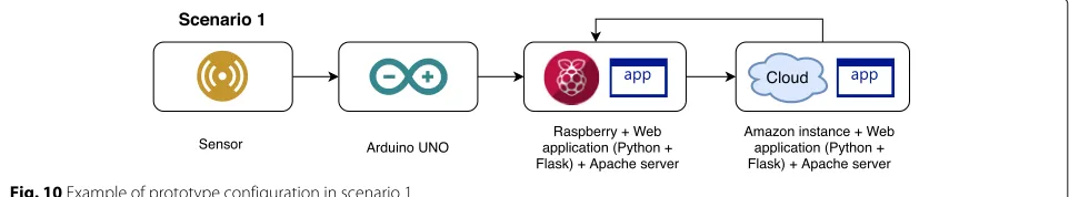
On the fog and cloud computing side, we configured a web application that receives and processes data from the edge device. This web application was implemented using Python and Flask13. In addition, we use Apache as a con-tainer for both applications. Figure10shows an example considering the scenario 1.
We use the same web application in scenarios 2 and 3, however the cloud and fog applications differ in scenario 1. In scenario 1, the fog application receives data from the Arduino and sends the data to the cloud application. After it receives a cloud response, the fog device returns a response to the Arduino. In scenarios 2 and 3, the cloud and fog applications receive and process requests directly
Table 8Indexes of the three paramaters that affect more the metric of each scenario
Scenario 1 Scenario 2 Scenario 3
Parameter Index Parameter Index Parameter Index
MTTF_Fog 2.64×10⁻⁴ MTTF_Cloud 1.95×10⁻⁴ MTTF_Fog 2.65×10⁻⁴
MTTR_Fog 2.57×10⁻⁴ MTTR_Cloud 1.93×10⁻⁴ MTTR_Fog 2.57×10⁻⁴
MTTF_Cloud 1.95×10⁻⁴ MTTR_Sensors 3.57×10⁻⁵ MTTR_Sensors 3.57×10⁻⁵
from the Arduino and send back a confirmation response to the Arduino platform.
Prototype measurement methodology and results
To recap, we have now defined three different
scenar-ios (Fig. 4), and have two different fog devices, two
different network connections, and four different cloud geo-locations. Furthermore, for each scenario we have multiple configurations.
Figure 11 shows the methodology used to setup
the devices according to each scenario used in our
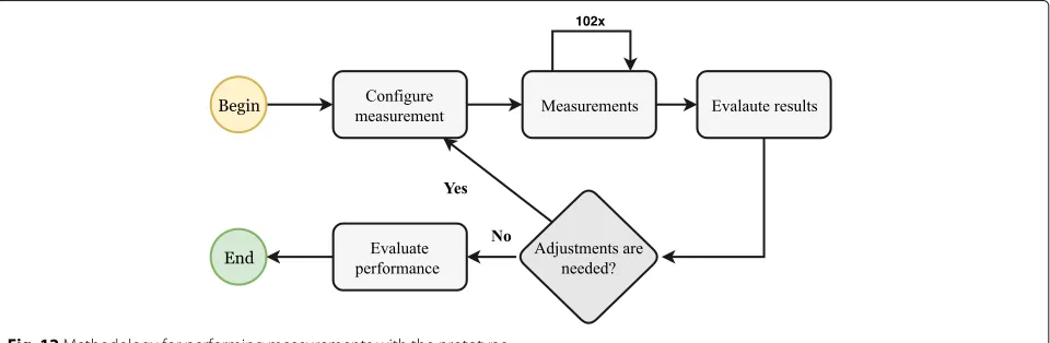
experiments, while Fig.12shows the methodology used
to perform the experiments. Note: the interval between requests was set up to 2 s, totaling 102 requests for each experiment.
Table6shows the average time (and the standard devi-ation) obtained from our measurements. In scenario 1, one can see that the geographic location of the cloud
Fig. 15Availability results of scenario 2 varyingathe cloud MTTF,bthe cloud MTTR andc, the sensor MTTR
instances impacts performance. For example, the Net-book connected to the São Paulo instance using the Ethernet option had a mean delay of 197.84 ms, while the mean service time for the Tokyo instance was 586.02 ms. In this case, there is an increase of 196.20% due to geographical distance. As expected, the connection type also impacted delay. For example, with the Net-book connected to the cloud instance located in São Paulo, the delay increases 31.83% when we changed the Ethernet connection to IEEE 802.11 (from 197.84 ms to 260.81 ms respectively). However, when the Rasp-berry Pi was used as a fog device, the impact of the network connection was less. Delay from the Raspberry Pi using the Ethernet to a cloud instance located in São Paulo was 207.15 ms, while using IEEE 802.11 was 215.61 ms, an increase of only 3.92%. The largest impacts recorded related to the Netbook can be explained by the network card.
In scenario 2, the same geographic impact is noted as per scenario 1. However, once there is a direct connec-tion between the microcontroller (Arduino) and the cloud
instances, the delay is lower than scenario 1 since there is an intermediary fog node. As expected, the greater the dis-tance from the microcontroller to the cloud insdis-tance, the longer the delay. From an instance located in São Paulo to an instance located in Tokyo, the delay increased 215.45% from 179.76 ms to 567.06 ms.
Scenario 3 behaves similarly to scenario 1 regarding network connection impact. The mean delay from the microcontroller to the Netbook through an Ethernet con-nection was 66.14 ms, while through IEEE 802.11 was, on average, 76.37 ms, an increase of 15.46%. The Raspberry Pi mean delay was similar, from 67.77 ms to 75.50 ms (increase of 11.40%) using the Ethernet and IEEE 802.11 network connection respectively.
Fig. 16Availability results of scenario 3 varyingathe fog MTTF,bthe fog MTTR andc, the sensor MTTR
Table 9Performance results of scenario 1
Fog device→Network connection→Cloud geo-location Throughput (requests/year) Service Time (ms)
Netbook→Ethernet→São Paulo 15,738,041.69 1851.17
Netbook→Ethernet→California 15,736,826.80 2300.51
Netbook→Ethernet→London 15,736,728.23 2352.86
Netbook→Ethernet→Tokyo 15,736,220.39 2664.78
Netbook→IEEE 802.11→São Paulo 15,737,640.90 1962.35
Netbook→IEEE 802.11→California 15,736,364.61 2567.16
Netbook→IEEE 802.11→London 15,736,259.12 2635.18
Netbook→IEEE 802.11→Tokyo 15,735,924.73 2890.17
Raspberry Pi→Ethernet→São Paulo 15,737,979.44 1867.21
Raspberry Pi→Ethernet→California 15,736,792.77 2318.46
Raspberry Pi→Ethernet→London 15,736,760.02 2332.73
Raspberry Pi→Ethernet→Tokyo 15,736,212.84 2671.46
Raspberry Pi→IEEE 802.11→São Paulo 15,737,907.39 1881.88
Raspberry Pi→IEEE 802.11→California 15,736,725.89 2354.14
Raspberry Pi→IEEE 802.11→London 15,736,664.17 2386.73
Fig. 17Scenario 2 performance results:athroughput, andbservice time
high standard deviation average service time when com-pared to the Ethernet connection. This can be explained by interference with physical objects, high loss package, and collision avoidance mechanism present in wireless connections [52].
Results from stochastic models and discussions
In this section, we present and discuss the results for both availability and performance obtained from our models.
Availability results
To perform analysis on our models, we collected each component’s MTTF and MTTR values in line with extant literature. The MTTF and MTTR values of fog device
hardware (HW_Fog) were estimated through an average
of HW values found in [39, 53–56], because the val-ues for the specific hardware used was not available. All values we used to set our models are described in Table7.
The availability and downtime results for each scenario are presented in Fig.13. Scenario 2 presents the best avail-ability level (0.9987%) in comparison with the scenario 1 (0.9973%) and 3 (0.9983%). This means that scenario 2 presents 11.01 h/year of downtime, while scenario 3 has 15.20 h/year, and scenario 1, 23.65 h/year. Scenario 1
Table 10Performance results of scenario 2
Cloud geo-location Throughput (requests/year) Service Time (ms)
São Paulo 15,758,748.10 2319.58
California 15,758,746.89 2830.46
London 15,758,746.81 2861.87
Tokyo 15,758,745.88 3252.77
presents the lowest availability because all the compo-nents are in series; all compocompo-nents are essential to e-health monitoring system operation.
Sensitivity analysis
For the sensitivity analysis, we used the MTTF and MTTR values from our system’s components as parameters, vary-ing them in ten values within a range defined by maximum and minimum values (10% plus and minus the default value). Table8shows the top three components (and their respective sensitivity index) that most impact on system availability.
Figure 14 represents the availability variation of the top three parameters that most impact system availabil-ity in scenario 1. As expected, when we increase the MTTF value (see Fig. 14a and c), the availability also increases, but in this case, the fog device MTTF has more impact than the cloud MTTF. An increase of 20% in fog device MTTF results in a notional reduction of 2.1051 h in annual downtime, while the same increase in cloud MTTF results in a smaller decrease in downtime i.e. only 1.4088 h.
Fig. 18Scenario 3 performance results:athroughput, andbservice time
same increase in the sensor’s MTTR results in a decrease of 0.0312 h.
Performance results
We perform stationary analysis on our performance model. The service time used in the analysis was set up with delays measured through our prototype experiments (Table6), while the time to arrival requests was set up 2 s. Table9presents the performance results obtained from the analysis of our model. One can note that changing the geographic location of the cloud instance impacts the per-formance metrics evaluated. For example, let’s consider the Netbook sending data using the Ethernet. To send data to the cloud instance located in São Paulo, the throughput was 15,738,041.69 requests/year. To send to the instance located in Tokyo was 15,736,220.39 requests/year. In this same configuration, the service time increases from 1851.17 to 2664.78 ms.
The change of connection type had a low impact on the metrics evaluated. For instance, for messages sent from the Netbook to the instance located in São Paulo, the throughput using the Ethernet and IEEE 802.11 were 15,738,041.69 requests/year and 15,737,640.90 requests/year respectively; the service times were 1851.17 and 1962.35 ms respectively. In general and as expected, the Netbook had a superior performance than the Rasp-berry Pi due to its superior hardware configuration.
Figure17and Table10present the results of scenario 2. As in scenario 1, the geographic locations of cloud instances also impacted on the performance metrics. The throughput for the instance located in São Paulo was 15,758,748.10 requests/year and decreased as the distance of the instance location increased, reaching 15,758,745.88 requests/year for the instance located in Tokyo. The ser-vice time is also impacted, from 2319.58 ms for the instance located in São Paulo and 3252.77 ms for instance located in Tokyo.
Finally, Fig. 18and Table 11present the performance results for scenario 3. In this scenario, a significant impact was identified relating to the type of network connection. For example, the throughput of the Netbook using the Ethernet was 15,748,129.90 requests/year,
while through IEEE 802.11 was 15,748,129.83
requests/year. A similar impact was identified with the service time i.e. 2842.23 and 2856.60 ms. The Netbook and Raspberry Pi display similar behaviors as they both experienced a close delay in prototype experiments.
The processing capacity of the fog device
(place 3_Fog_Capacity) and cloud server (place
3_Cloud_Capacity) was limited in our models (600 and 1000, respectively) to avoid state explosion when solving the model analytically. Nonetheless, we noted that increasing the capacity to process simultaneous
Table 11Performance results of scenario 3
Fog device→Network connection Throughput (requests/year) Service Time (ms)
Netbook→Ethernet (N-E) 15,748,129.90 2842.23
Netbook→IEEE 802.11 (N-I) 15,748,129.83 2856.60
Raspberry Pi→Ethernet (R-E) 15,748,129.89 2844.51
requests substantially neither affects the throughput nor the service time metrics. For values greater than 600 and 1000, the impact on analyzed metrics were almost insignificant. For instance in scenario 2, when we set fog and cloud capacity as 600 and 1000 respec-tively, the Markov chain was composed of 24,032 states and the result was 1799.3254 requests/hour and 1269.2155 ms for throughput and service time respec-tively. When we use 1200 and 2000, the Markov chain was composed of 48,032 states resulting in 1799.4367
requests/hour and 1412.8086 ms for throughput
and service time respectively).
Discussions
From the stationary analysis, we evaluated availabil-ity in each scenario. We noted that the best avail-ability level (0.9987%) was achieved in scenario 2 (where only the cloud application is considered) and the worst one (0.9973%) was scenario 1 (using both fog and cloud). It is an interesting result since in scenario 1 we have more computational layers and con-sequently more devices can fail (and thereby decreas-ing the availability of the whole system). Thus, despite the extension of fog node capability by the cloud, this integrated scenario is more complex and as a result has more points of failures despite the hypothesized benefits.
Regarding the sensitivity analysis results, there is greater variability in the components that impact the avail-ability of e-health monitoring system in the scenarios examined. In scenario 1, the most critical component is the fog device whereas in scenarios 2 and 3, the fog device and cloud infrastructure impact the system respectively. An increase of 20% in MTTF value of fog device (scenario 1) results in a reduction of 2.1051 h in annual downtime. An increase of 20% in MTTF of cloud infrastructure results in reduction of 1.4108 h of annual downtime (scenario 2). And in scenario 3, an increase of 20% in MTTF of fog devices results in reduc-tion of 2.1071 h of annual downtime. Depending on the configuration chosen for the e-health monitoring sys-tem, investments can be made to increase availability, or by adding more redundant equipment provide greater reliability.
Within the prototype experiments, we noted an increase of delay as the distance from microcontroller/fog devices to cloud instance increases both in scenario 1 and 2, as expected. The delay in scenario 1 was slightly higher than scenario 2 once the fog devices are added. However, the addition of fog devices (sce-nario 1) enables the pre-analysis of data collected by sensors before sending to the cloud. Thus, simple deci-sions, such as calling an ambulance, can be made quicker.
We also observed that the delay to send data from microcontroller to fog devices is significantly lower than sending to the cloud. Considering the closer proximity of the the cloud instance to the microcontroller (São Paulo), the mean delay was 179.76 ms, while the higher mean delay to send to the cloud was 76.37 ms (Netbook with IEEE 802.11). For delay-sensitive systems (e.g. e-health monitoring systems, augmented reality, real-time video analytics, and content delivery [22]), fog devices can greatly reduce the delay and increase the performance of these systems. However, one should not disregard the limited computing capacity of these devices.
These experiment results were used to feed the perfor-mance model. For scenarios 1 and 2, as the geographic distance of the cloud instance increases, the throughput decreases (see Tables 9 and10). Once the time to pro-cess a request increases, fewer requests will be propro-cessed because they will remain in the queue for longer (see Fig.8). In addition, service time is directly impacted by the geographic location of an instance i.e. the longer it takes to send the request, the longer it will take to pro-cess the request and to receive a response. For an e-health monitoring application, where some decisions need to be made quickly, hosting the cloud instance in a remote geo-graphic region may have a significant impact on service time and associated QoS levels.
Scenario 1 had the lowest availability level and the worst performance results. This can be explained as follows. The e-health system is considered operational only when all components of the scenario are working and this reduces the availability of the system as a whole. Relatively poor performance results are due to the high delay in send-ing data from the microcontroller to the cloud passsend-ing through a fog device. Notwithstanding this, this scenario can take advantage of the computing capacity and virtually unlimited data storage that cloud computing offers.
Scenario 2 presented the best availability level and bet-ter performance results than others. The improvement in performance is due to the decrease in delay because the data is sent directly from the microcontroller to the cloud (without fog devices). Notwithstanding this, the delay in scenario 2 can compromise systems that are delay-sensitive.
Conclusions
Fog and cloud computing address a number of problems encountered in IoT however they also increase manage-ment complexity. Despite fog and cloud computing offer-ing greater availability and resilience, they can also be viewed as vulnerabilities or potential points of failure. As such, in addition to edge device failure, attention must be paid to fog node and cloud infrastructure failures. While cloud and fog integration is relatively well known and shares common technologies, the integration/extension with IoT is a non-trivial task, mostly due to massive device heterogeneity and service requirements.
Some systems have high criticality and any downtime can lead in extreme cases to death as in the case of an e-health monitoring system, the focus of this article. The main goal of the is study was to identify the bottlenecks in an integrated e-health monitoring system and propose strategies to minimize the application downtime, prevent failures, and guide financial investment decision making.
In this paper, we proposed an architecture to pro-vide an e-health monitoring system relying on IoT sen-sors, fog devices and cloud infrastructure. This service was evaluated regarding its availability and performance. We proposed stochastic models by using SPN and RBD approaches. To use realistic data as an input to our mod-els, we also developed and implemented a prototype with different types of fog device, network connection, and cloud instances located in four different geographic loca-tions.
From our results, it is clear that there is a trade-off between performance and service time. In this way, it is necessary to prioritize the application requirements before deciding on the best architecture. This is illus-trated by the results from the various scenarios. For example, the scenario that relies only on cloud infras-tructure (scenario 2) presents the best availability level since cloud providers can offer a better service as mea-sured by reliability than fog devices. On the other hand, scenario 1, which relies on fog devices and cloud infras-tructure, may be more appropriate to host e-health mon-itoring systems due to the technological limitations of end-devices. Other configurations may be more appro-priate depending on the use scenario e.g. big data services.
As future works, we plan to analyze the impact of redundancy and understand how we can improve the availability of the system by adding more cloud servers or fog devices. We also plan to evolve the prototype system with different types of smart-end devices, fog devices, and analytical techniques (including machine learning) to treat the vital signs data from patients and analyze the impact of processing data on fog devices and cloud servers. Finally, we intend to evaluate dif-ferent IoT communication protocols, such as MQTT,
COAP, and AMQP with the goal of improving the prototype and measuring different metrics such as the QoS of application.
Endnotes 1https://www.sierrawireless.com 2https://www.raspberrypi.org/ 3https://www.arduino.cc/ 4 http://www.nvidia.com/object/deep-learning-in-medicine.html 5http://www.modcs.org/?p=2264
6The metric descriptions follow the Mercury tool
syn-tax. 7https://github.com/WorldFamousElectronics/ PulseSensor_Amped_Arduino 8https://www.arduino.cc/ 9https://www.arduino.cc/en/Guide/ ArduinoEthernetShield 10http://mqtt.org/ 11 https://www.raspberrypi.org/products/raspberry-pi-3-model-b/ 12www.aws.amazon.com/ec2
13Flask is a microframework for building web
applica-tions using the Python language. See http://flask.pocoo. org/docs/0.12/
Abbreviations
AT: Arrival time; AWS: Amazon web services; BPM: Beat per minute; EC2: Elastic compute cloud; IBB: Interval between beats; IoT: Internet of things; ms: Milliseconds; MTTF: Mean time to failure; MTTR: Mean time to repair; RBD: Reliability diagram blocks; SPN: Stochastic petri nets; ST: Service time
Acknowledgments
The authors would like to thank Universidade de Pernambuco, CNPq (Conselho Nacional de Desenvolvimento Científico e Tecnológico) and CAPES (Coordenação de Aperfeiçoamento de Pessoal de Nível Superior) for supporting this work.
This work is partially funded by the European Union’s Horizon 2020 Research and Innovation Programme through RECAP (http://www.recap-project.eu) under Grant Agreement Number 732667.
Funding
This work is partially funded by the European Union’s Horizon 2020 and FP7 Research and Innovation Programmes through RECAP ( http://www.recap-project.eu) under Grant Agreement No. 732667.
Availability of data and materials
Not applicable
Authors’ contributions
Competing interests
The authors declare that they have no competing interests.
Publisher’s Note
Springer Nature remains neutral with regard to jurisdictional claims in published maps and institutional affiliations.
Author details
1Universidade Federal de Pernambuco (UFPE), Grupo de Pesquisa em Redes
de Computadores e Telecomunicações (GPRT), Recife, Pernambuco, Brazil.
2Universidade de Pernambuco (UPE), Recife, Pernambuco, Brazil.3Dublin City
University (DCU), Irish Centre for Cloud Computing and Commerce (IC4), Dublin, Ireland.
Received: 12 March 2018 Accepted: 22 August 2018
References
1. Islam SR, Kwak D, Kabir MH, Hossain M, Kwak K-S (2015) The internet of things for health care: a comprehensive survey. IEEE Access 3: 678–708
2. Atzori L, Iera A, Morabito G (2010) The internet of things: A survey. Comput Netw 54(15):2787–2805
3. Biswas AR, Giaffreda R (2014) Iot and cloud convergence: Opportunities and challenges. In: Internet of Things (WF-IoT), 2014 IEEE World Forum On. IEEE. pp 375–376. https://www.computer.org/csdl/proceedings/wf-iot/2014/3459/00/06803194-abs.html
4. Botta A, De Donato W, Persico V, Pescapé A (2014) On the integration of cloud computing and internet of things. In: Future Internet of Things and Cloud (FiCloud), 2014 International Conference On. IEEE. pp 23–30.
https://ieeexplore.ieee.org/abstract/document/6984170/
5. Lee I, Lee K (2015) The internet of things (iot): Applications, investments, and challenges for enterprises. Bus Horiz 58(4):431–440
6. Vaquero LM, Rodero-Merino L (2014) Finding your way in the fog: Towards a comprehensive definition of fog computing. ACM SIGCOMM Comput Commun Rev 44(5):27–32
7. Bonomi F, Milito R, Zhu J, Addepalli S (2012) Fog computing and its role in the internet of things. In: Proceedings of the First Edition of the MCC Workshop on Mobile Cloud Computing. ACM. pp 13–16.https://dl.acm. org/citation.cfm?id=2342513
8. Mell P, Grance T The NIST definition of cloud computing. NIST Special Publication 800-145. 2011.http://faculty.winthrop.edu/domanm/csci411/ Handouts/NIST.pdf
9. Mshali H, Lemlouma T, Magoni D (2018) Adaptive monitoring system for e-health smart homes. Pervasive Mob Comput 43:1–19
10. Trivedi K, Andrade E, Machida F (2012) Combining performance and availability analysis in practice. In: Advances in Computers vol 84. Elsevier. pp 1–38.https://www.sciencedirect.com/science/article/pii/
B9780123965257000010
11. Zeng W, Koutny M, Watson P (2015) Opacity in internet of things with cloud computing (short paper). In: Service-Oriented Computing and Applications (SOCA), 2015 IEEE 8th International Conference On. IEEE. pp 201–207.https://ieeexplore.ieee.org/abstract/document/ 7399111/
12. Colom JF, Mora H, Gil D, Signes-Pont MT (2017) Collaborative building of behavioural models based on internet of things. Comput Electr Eng 58:385–396
13. Lomotey RK, Pry J, Sriramoju S (2017) Wearable iot data stream traceability in a distributed health information system. Pervasive Mob Comput 40:692–707
14. Araujo J, Silva B, Oliveira D, Maciel P (2014) Dependability evaluation of a mhealth system using a mobile cloud infrastructure. In: Systems, Man and Cybernetics (SMC), 2014 IEEE International Conference On. IEEE. pp 1348–1353.https://ieeexplore.ieee.org/abstract/document/6974102/
15. Li Y, Orgerie A-C, Rodero I, Parashar M, Menaud J-M (2017) Leveraging renewable energy in edge clouds for data stream analysis in iot. In: Proceedings of the 17th IEEE/ACM International Symposium on Cluster, Cloud and Grid Computing. IEEE Press. pp 186–195.https://ieeexplore. ieee.org/abstract/document/7973702/
16. Souza VB, Masip-Bruin X, Marin-Tordera E, Ramírez W, Sanchez S (2016) Towards distributed service allocation in fog-to-cloud (f2c) scenarios. In: Global Communications Conference (GLOBECOM), 2016 IEEE. IEEE. pp 1–6.https://ieeexplore.ieee.org/abstract/document/7842341/
17. Bradley J, Reberger C, Dixit A, Gupta V (2013) Internet of everything: A $4.6 trillion public-sector opportunity. Whitepaper.https://www.cisco. com/c/dam/en_us/about/businessinsights/docs/ioe-public-sector-vas-white-paper.pdf
18. Bradley J, Barbier J, Handle D (2013) Embracing the Internet of Everything To Capture Your Share of $14.4 Trillion. Whitepaper.https://www.cisco. com/c/dam/en_us/about/ac79/docs/innov/IoE_Economy.pdf
19. Shi W, Cao J, Zhang Q, Li Y, Xu L (2016) Edge computing: Vision and challenges. IEEE Internet Things J 3(5):637–646
20. Chiang M, Zhang T (2016) Fog and iot: An overview of research opportunities. IEEE Internet Things J 3(6):854–864
21. Iorga M, Feldman L, Barton R, Martin MJ, Goren N, Mahmoudi C The NIST Definition of Fog Computing. NIST Special Publication 800-191 (Draft). 2017.https://csrc.nist.gov/csrc/media/publications/sp/800-191/draft/ documents/sp800-191-draft.pdf
22. Yi S, Li C, Li Q (2015) A survey of fog computing: concepts, applications and issues. In: Proceedings of the 2015 Workshop on Mobile Big Data. ACM. pp 37–42.https://dl.acm.org/citation.cfm?id=2757397
23. Luan TH, Gao L, Li Z, Xiang Y, Wei G, Sun L (2015) Fog computing: Focusing on mobile users at the edge. arXiv preprint arXiv:1502.01815.
https://arxiv.org/abs/1502.01815
24. Gissler B, Shrivastava P (2015) A system for design decisions based on reliability block diagrams. In: Reliability and Maintainability Symposium (RAMS), 2015 Annual. IEEE. pp 1–6.https://ieeexplore.ieee.org/abstract/ document/7105105/
25. Hasan O, Ahmed W, Tahar S, Hamdi MS (2015) Reliability block diagrams based analysis: A survey. In: AIP Conference Proceedings, vol 1648. AIP Publishing. p 850129.https://aip.scitation.org/doi/abs/10.1063/1.4913184
26. Signoret J-P, Dutuit Y, Cacheux P-J, Folleau C, Collas S, Thomas P (2013) Make your petri nets understandable: Reliability block diagrams driven petri nets. Reliab Eng Syst Saf 113:61–75
27. Bourouni K (2013) Availability assessment of a reverse osmosis plant: comparison between reliability block diagram and fault tree analysis methods. Desalination 313:66–76
28. Dantas J, Matos R, Araujo J, Maciel P (2015) Eucalyptus-based private clouds: availability modeling and comparison to the cost of a public cloud. Computing 97(11):1121–1140
29. Labadi K, Benarbia T, Barbot J-P, Hamaci S, Omari A (2015) Stochastic petri net modeling, simulation and analysis of public bicycle sharing systems. IEEE Trans Autom Sci Eng 12(4):1380–1395
30. Li P, Yang C, Xu H, LAU TF, Wang R (2017) User behaviour authentication model based on stochastic petri net in cloud environment. In: International Symposium on Parallel Architecture, Algorithm and Programming. Springer. pp 59–69.https://link.springer.com/chapter/10. 1007/978-981-10-6442-5_6
31. Almutairi LM, Shetty S (2017) Generalized stochastic petri net model based security risk assessment of software defined networks. In: Military Communications Conference (MILCOM), MILCOM 2017-2017 IEEE. IEEE. pp 545–550.https://ieeexplore.ieee.org/abstract/document/8170813/
32. Heidary Z, Ghaisari J, Moein S, Naderi M, Gheisari Y (2016) Stochastic petri net modeling of hypoxia pathway predicts a novel incoherent
feed-forward loop controlling sdf-1 expression in acute kidney injury. IEEE Trans Nanobioscience 15(1):19–26
33. Pianosi F, Beven K, Freer J, Hall JW, Rougier J, Stephenson DB, Wagener T (2016) Sensitivity analysis of environmental models: A systematic review with practical workflow. Environ Model Softw 79:214–232
34. Razavi S, Gupta HV (2015) What do we mean by sensitivity analysis? the need for comprehensive characterization of “global” sensitivity in earth and environmental systems models. Water Resour Res 51(5):3070–3092 35. Hamby D (1994) A review of techniques for parameter sensitivity analysis
of environmental models. Environ Monit Assess 32(2):135–154
36. Chiuchisan I, Costin H-N, Geman O (2014) Adopting the internet of things technologies in health care systems. In: Electrical and Power Engineering (EPE), 2014 International Conference and Exposition On. IEEE.
pp 532–535.https://ieeexplore.ieee.org/abstract/document/6969965/
38. Matos R, Araujo J, Oliveira D, Maciel P, Trivedi K (2015) Sensitivity analysis of a hierarchical model of mobile cloud computing. Simul Model Pract Theory 50:151–164
39. Matos R, Dantas J, Araujo J, Trivedi KS, Maciel P (2017) Redundant eucalyptus private clouds: Availability modeling and sensitivity analysis. J Grid Comput 15(1):1–22
40. Jain R (1990) The Art of Computer Systems Performance Analysis: Techniques for Experimental Design, Measurement, Simulation, and Modeling. John Wiley & Sons.https://www.wiley.com/en-us/The+Art+ of+Computer+Systems+Performance+Analysis%3A+Techniques+for+ Experimental+Design%2C+Measurement%2C+Simulation%2C+and+ Modeling-p-9780471503361
41. Rahmati SHA, Ahmadi A, Sharifi M, Chambari A (2014) A multi-objective model for facility location–allocation problem with immobile servers within queuing framework. Comput Ind Eng 74:1–10
42. Vilaplana J, Solsona F, Teixidó I, Mateo J, Abella F, Rius J (2014) A queuing theory model for cloud computing. J Supercomput 69(1):492–507 43. Pham TN, Tsai M-F, Nguyen DB, Dow C-R, Deng D-J (2015) A cloud-based
smart-parking system based on internet-of-things technologies. IEEE Access 3:1581–1591
44. Al-Haidari F, Sqalli M, Salah K (2015) Evaluation of the impact of edos attacks against cloud computing services. Arab J Sci Eng 40(3): 773–785
45. Adhikary T, Das AK, Razzaque MA, Alrubaian M, Hassan MM, Alamri A (2017) Quality of service aware cloud resource provisioning for social multimedia services and applications. Multimedia Tools Appl 76(12):14485–14509
46. Goldsztajn D, Ferragut A, Paganini F, Jonckheere M (2018) Controlling the number of active instances in a cloud environment. ACM SIGMETRICS Perform Eval Rev 45(2):15–20
47. Yang B, Tan F, Dai Y-S, Guo S (2009) Performance evaluation of cloud service considering fault recovery. In: IEEE International Conference on Cloud Computing. Springer. pp 571–576.https://link.springer.com/ chapter/10.1007/978-3-642-10665-1_54
48. Khazaei H, Misic J, Misic VB (2012) Performance analysis of cloud computing centers using m/g/m/m+ r queuing systems. IEEE Trans Parallel Distrib Syst 23(5):936–943
49. Shelby Z, Hartke K, Bormann C (2014) The constrained application protocol (CoAP). No. RFC 7252. 2014.http://www.rfc-editor.org/info/ rfc7252,https://doi.org/10.17487/RFC7252
50. Shang W, Yu Y, Droms R, Zhang L (2016) Challenges in iot networking via tcp/ip architecture. Technical Report NDN-0038. NDN Project
51. Chen X, Huang X, Jiao C, Flanner MG, Raeker T, Palen B (2017) Running climate model on a commercial cloud computing environment: A case study using community earth system model (cesm) on amazon aws. Comput Geosci 98:21–25
52. Sagari S, Seskar I, Raychaudhuri D (2015) Modeling the coexistence of lte and wifi heterogeneous networks in dense deployment scenarios. In: Communication Workshop (ICCW), 2015 IEEE International Conference On. IEEE. pp 2301–2306.https://ieeexplore.ieee.org/abstract/document/ 7247524/
53. Araujo J, Maciel P, Torquato M, Callou G, Andrade E (2014) Availability evaluation of digital library cloud services. In: Dependable Systems and Networks (DSN), 2014 44th Annual IEEE/IFIP International Conference On. IEEE. pp 666–671.https://ieeexplore.ieee.org/abstract/document/ 6903622/
54. Silva B, Maciel P, Tavares E, Zimmermann A (2013) Dependability models for designing disaster tolerant cloud computing systems. In: Dependable Systems and Networks (DSN), 2013 43rd Annual IEEE/IFIP International Conference On. IEEE. pp 1–6.https://ieeexplore.ieee.org/abstract/ document/6575323/
55. Tang D, Kumar D, Duvur S, Torbjornsen O (2004) Availability measurement and modeling for an application server. In: Dependable Systems and Networks, 2004 International Conference On. IEEE. pp 669–678.https://ieeexplore.ieee.org/abstract/document/1311937/
56. Kim DS, Machida F, Trivedi KS (2009) Availability modeling and analysis of a virtualized system. In: Dependable Computing, 2009. PRDC’09. 15th IEEE Pacific Rim International Symposium On. IEEE. pp 365–371.https:// ieeexplore.ieee.org/abstract/document/5368189/
57. Novacek G Tips for Predicting Product Reliability.http://circuitcellar.com/ cc-blog/tips-for-predicting-product-reliability/. Accessed 05 Jan 2018