A New Fuzzy Hybrid Dynamic Programming for Scheduling Weighted Jobs on Single Machine

A New Fuzzy Hybrid Dynamic Programming for Scheduling

Weighted Jobs on Single Machine

Seyedeh Maedeh Mirmohseni

, Seyed Hadi Nasseri

, Mohammad Hossein Khaviari

1_{Department of Mathematics and Information Science, Guangzhou University, Guangzhou, China} 2 _{Department of Mathematics, University of Mazandaran, Babolsar, Iran}

3_{Department of Industrial Engineering, Mazandaran University of Science and Technology, Babol,} Mazandaran, Iran

A B S T R A C T P A P E R I N F O

In this paper, dynamic programming for sequencing weighted jobs on a single machine to minimizing total tardiness is focused, to significance of fuzzy numbers field, and importance of that for decision makers who are facing on uncertain data, combination of dynamic programming and fuzzy numbers is applied. A random scheduling problem with fuzzy processing times is given and solved. In addition, algorithm consuming time during solving same category problem and different sizes are analyzed that for large problem CPU time usage is extremely unaffordable. Therefore demonstration of near-exact heuristic method such as Genetic Algorithm (GA) appears. In this paper sufficient discussion around solving this kind of problems and their algorithms analysis and a combination between Dynamic Programming (DP) and genetic algorithm as a newly born method is proposed that stand on DP performance and genetic algorithm search power, and finally comparison on the recent developed method has been held. Then this method can deal with real-world problem easily. Thus, decision makers actually can use this modification of dynamic programming for coping with un-crisp problem.

Chronicle:

Received: 04 June 2017 Revised: 01 August 2017 Accepted:10 August 2017 Available:10 August 2017

Keywords :

Comparing Fuzzy Numbers. Dynamic Programming. Genetic Algorithm. Scheduling.

1. Introduction

Dynamic Programming (DP) is a constructional method on solving an Optimization Problem (OP). In dynamic programming for solving OP, main problem will be partitioned into several sub-problems and after this action, these sub-problems can be solved as an Independent Partial Optimization Problem (IPOP), and eventually with connecting these IPOP solutions, main solution of original problem could be gained.

 _{Corresponding author}

E-mail address: [email protected] DOI: 10.22105/jarie.2017.49214

Journal of Applied Research on Industrial

Engineering

In fact, this method uses divide-and-conquer approach to come along:  It divides main problem into IPOP.

 It solves IPOP’s in recursive manner.  IPOP’s solutions will be tailored together.

DP is a general optimization technique for making sequential decisions. Here we have to decide which job comes first, which comes second, and so on. Dynamic Programming applies to problems that can be partitioned into sub-problems, each involving a subset of the decisions, in such a way that the following optimalityprinciple holds: suppose we have already made the first k sequences (optimally or not), then the remaining (n-k) sequences can be optimized by considering only the sub-problem that involves them explained by [1].

DP can solve prevalent sort of OP, But in real world problems managers or decision makers face with crisp and certain data in rare, so developing this method (e.g., [2- 4]) across fuzzy field can be interesting point of view for them. The concept of decision making in fuzzy environment was first proposed by Bellman and Zadeh [5], then in Fuzzy Dynamic Programming (FDP), Kacprzyk and Esogbue [6] developed fundamental concept first time and they did something in expertizing it.

DP has become a standard tool in many areas (e.g., control, operations research, systems analysis, data analysis) considerable advances have been made in the theoretical developments of DP, and even the thorny problems of its computation efficiency have been alleviated in many cases. Numerous of application to real-life problem e.g., vehicle routing [7], manufacturing [8], etc. have been recently reported. Numerous contributions to FDP of both a foundational [9-11] and applied character (e.g., [12]). Scheduling ‘n’ weighted jobs on a single machine is the kind of OPs that can be solved by DP.

Genetic Algorithm first introduced by John Holland [13], Genetic Algorithm (GA) is a search algorithm based on the conjecture of natural selection and genetics. The features of Genetic Algorithm are different from other search techniques in several aspects. First, algorithm is a multi-path that searches many peaks in parallel, hence reducing the possibility of local minimum trapping. Second, the GA works with a coding of parameters instead of the parameters themselves and by this computational time decreases rapidly. Third, the GA evaluates the fitness of each string to guide its search instead of the optimization function narrated by [14]. GA operates on a population of individuals. After an initial population randomly or heuristically is generated, the algorithm evolves the population through sequential and iterative application of three operators: selection, crossover and mutation. A new generation is formed at the end in each iteration [15].

population is generated and algorithm will be continued till reach convergence or stopping criteria. In Fig 1Pseudo-code of GA has been shown.

Combination of meta-heuristics and dynamic programming could be a brilliant idea if it held well. There are some survives around joining these two problem solvers together like [16] that did some effort to use benefits of these two methods, however each method can be used as sub-function and vice versa. In this article DP take part in main function and GA play recursively and in iterative manner. So in this structure ability of both methods could be gained.

Algorithm 1. Pseudo-code of GA Initializing problem {Popsize, Iteration, Pc, Pm} Intpop= Initial-population-Generators ();

Sort pop= Sortpop(1); Pop2 Intpop; While q<iteration && z< Max non-developed

For i=1 to Posize If (cross over happens)

Pop1 crossover(Mating pool) Break;

If (mutation happens)

Pop1 Mutation(Mating pool)

Break;

If (Reproduction happens)

Pop2 Copy(Mating pool) Pop2 Pop1;

Stopping criteria check();

End

End

Hybridization between heuristic methods and DP categories has been happened before in some cases, [17] hybridized GA and DP to coping with long-term generation expansion planning problem, [18] proposed using simulated annealing and DP to solve unit commitment problem, [19] proposed a DP-based heuristic method on dealing with slab stack shuffling problem, but dealing with scheduling problems by use of this hybridization as an approximation method to reduce dimensionality and computational time had been remained in some case of interest before something did in this article.

and due dates on a single machine. Jorge and Valente [31] proposed Several dispatching heuristics for single machine earliness/tardiness scheduling problem. A novel hybrid metaheuristic named as PHVNS proposed by [32] to solve restrictive single-machine earliness/tardiness scheduling problem (RSMETP), [33] worked on single machine total weighted tardiness problem as genetic algorithm for problem solver, a two-phase heuristic algorithm proposed by [34] for solving scheduling jobs on a single machine that requires periodic maintenance with the objective of minimizing the number of tardy jobs , Panneerselvam [35] proposed a simple heuristic, and Yoon and Lee [36] introduced constructive heuristics], they compared proposed method with famous present constructive methods, such as WCOVERT, ATC, WMDD that their heuristics perform much better. Recent two methods will be used in comparison circumstance.

2. Exact scheduling ‘n’ weighted jobs on a single machine with

T

criteria

I. Notation:

J

J



q_J : starting point of the job that in each stage can be in the beginning of its schedule:





J j

j

J

t

q

II. Recursive equations

Let G(J) be minimum cost of jobs in

J

    

  



j j

j j j

j j

j j

d c

d c w

d c c g

; 0

; *

) ( )

( (2)

By consideration above, recursive equation can be defined as following:





   



   



0 ) (

}) { ( ) (

min ) (



G

j J G t q g J

G j J j

J

j ₍₃₎

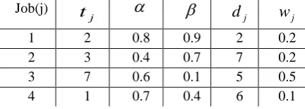
Table 1. Four weighted jobs with their specifications

According to(2)and(3), some fuzzy operations must be defined. Assume that (a,









be two triangular fuzzy numbers, summation, and deduction operations can be defined as following: (when a and b aremode of these numbers)

) , ,

(a  +(b,,)=(ab,,), (4) )

, ,

(a  (b,,)=(ab,,).

For comparing two fuzzy numbers in formA~(a,b,





 



1

0

) ~ ~

( 5 . 0 ) ~

(A InfA SupA d



Where,A~_ {xR|~(x)}

A , andA~(x) is membership function of the supposed fuzzy number. The

current formula and for A~(a,b,,) it will reduced into:

. (6)

The above formula can be applied for also triangular number with considering

a

b

) , , (

~ _{ }

a

A can be assumed greater or equal than B~(b,,) if and only if (A~)(B~)(More details are given in [47]). With these two last operators, fuzzy DP can be launched in state of art.

) 345 . 0 , 3925 . 0 , 9 . 0 ( ) 38 . 1 , 57 . 1 , 6 . 3 ( * 25 .

0 



T . (7) Let we are in kthstep, So we must choose one job from unscheduled (n-k+1) jobs that must be determined from th

k 1)

(  step, so if all steps have been prepared, selection can be done. As it can be seen, Table 4 shows the first job of optimal schedule (i.e. job 1), Table 3 in column {2,3,4} identifies the next, so with looking at Table 2 column {2,4}, job 4 shows itself as third order in schedule, and in end job 2 is obviously last task to do. So the optimal schedule is 1-3-4-2 with optimal criteria.

Job(j) j

t





1 2 0.8 0.9 2 0.2

2 3 0.4 0.7 7 0.2

3 7 0.6 0.1 5 0.5

4 1 0.7 0.4 6 0.1

)] (

5 . 0 [

* 5 . 0 ) ~

(   





 A a b

Table 3. Combination of two jobs consist of their J

q and G(J)

3.

In

epth

omputation

For lunching our combined method in real-world problem we need a computer programming to solve these kind of problems. Order of exact algorithms to find an optimal solution is extensive and this algorithm is not out of statement. Hence if recursive structure of algorithm is being studied, the order can be figured out as follows for ‘m’ jobs scheduling:



( . (8)

Where, in last summation,

_











i

m

means total subset number of m jobs with i elements, and for every subset including i elements algorithm will be applied i times. In Algorithm 2, pseudo-code of the algorithm can be seen.

Jo

b(j) {1,2} {1,3}

{1,

4} {2,3} {2,

4} {3,4} J q (8/1.3/0.5) (4/1.1/1.1 ) (10/1/0 .8) (3/1.5/ 1.3) (9/1.4 /1) (5/1.2/1.6) J j

1 2 1 3 1 4 2 3 2 4 3 4

j g 1. 6/0. 42/0. 28 0. 8/0. 34/0. 24 0. 8/0. 38/0. 4 3/0. 85/0. 6 2/0. 36/0. 3 4 0. 5/0. 17/0. 12 -0. 2/0. 38/0. 4 2. 5/1. 05/0. 7 1/0. 36/0. 3 4 0. 4/0. 21/0. 14 3. 5/0. 9/0. 8 5 0/0. 19/0. 2 G(J -{j}) 1. 2/0. 5/0. 4 2 2. 2/0. 38/0. 42 4/1/ 1. 05 2. 2/0. 38/0. 42 0. 7/0. 25/0. 21 2. 2/0. 38/0. 42 4/1/ 1. 05 1. 2/0. 5/0. 4 2 0. 7/0. 25/0. 21 1. 2/0. 5/0. 4 2 0. 7/0. 25/0. 21 4/1/ 1. 05 G(J ) 2. 8/0. 92/0. 7 3/0. 72/0. 6 6 4. 8/1. 38/1. 45 5. 2/1. 23/1. 02 2. 7/0. 61/0. 55 2. 7/0. 55/0. 54 3. 8/1. 38/1. 45 3. 7/1. 55/1. 12 1. 7/0. 61/0. 55 1. 6/0. 71/0. 56 4. 2/1. 15/1. 06 4/1. 1 9/1. 2 5 α-cut 3. 93821 4. 25887 6. 91026 7.

51193 _3.8266

3. 84071 5. 52102 5. 19692 2. 42958 2.

Table 2 & 5. First and last stages correspondingly in left & middle

Algorithm 2. Pseudo code of dynamic programming on single machine DP {J, T, W}

Initializing Algorithm: J=jobs;

T= Fuzzy processing time; W= Job weight;

For ( the cardinal of current applied set) K (i) = qj + DP (set\ {J(i)}, T, W) End

Return (min(k))

For paraphrasing due dates, two factors are included, DDR and TF: DDR is Due Date Rang and TF is Tightness Factor of due dates and they will be selected from set {0.2, 0.4, 0.6, 0.8, and 1}. So due date for job ‘j’, d_j is chosen by selecting an integer d_j from uniform distribution [

DDR/2) + TF -(1 p DDR/2), -TF -(1

p  ], where ‘p’ is sum of all processing times. High value of DDR indicates wide range of due dates and low amount of TF shows that due dates are loose and every amount near to 1 indicates tight due dates.

Note: if (1-TF-DDR/2)0 then due dates will be selected from interval [1,p(1-TF+DDR/2)] Some randomly generated problem have been given to computer (CPU: Dual 2.1GHz 1Mb, RAM: 4 GB) and their average time usages have been calculated. Fig 1shows CPU times for some instances.

Job(j) {1,2,3,4}

J

q 0

J

j 1 2 3 4

j g 0 /0 .1 6 /0 .1 8 0 1 /0 .3 /0 .0 5 0 G(J -{j }) 3. 6/1. 41/1. 06 4. 6/1. 43/1. 57 3/1. 05/0. 75 3. 9/1. 85/1. 38 G (J) 3 .6 /1 .5 7 /1 .2 4 4. 6/1. 43/1. 57 4 /1 .3 5 /0 .8 3. 9/1. 85/1. 38 α-cut 5 .1 0 5 5 6 .6 6 8 3 8 5 .5 3 3 6 1 5 .5 1 0 2 3

Job(j) {1} {2} {3} {4}

J

q

j 1 2 3 4

j

g 2.2,

0. 38, 0. 42 1. 2/0. 5/0. 42 0. 8/0. 25/0. 21 0. 7/0. 25/0. 21

G(J-{j}) 0 0 0 0

G(J) 2.2,

0. 38, 0. 42 1. 2/0. 5/0. 42 4/1/ 1. 05 0. 7/0. 25/0. 21 α-cu t ev al u at io n 3. 14244 1.

Table 4. Combination of three jobs consist of their qJ _{and G(J)}

According to situation above, for large instances CPU times are unimaginable, and it make years or decades to be solved, however computer over flowing must be considered as another physical constrain. Thus, solving those large instances with exact algorithms is not logical and recommended most of the times as if it is not so important to use an exact solution. Now this question might be arisen that how can manager take decision when they are in resource limitation? In other side, in spite of exact algorithm to solve problems, some near-exact method (they are so-called as heuristic and Meta heuristic methods) prove themselves which Genetic Algorithm is one of the most famous, productive and flexible method. As it has been explained before GA puts solving problem in an iterative mode and in each iteration it comes closer to exact solution if it does not fall into a local optima. Fig 1,Illustrates average CPU time usages for several sizes of instances.

Fig 1. Average CPU time usages for several sizes of instance

Job(j) {1,2,3} {1,2,4} {2,3,4} {1,3,4}

J

q (1/0.7/0.4) (7/0.6/0.1) (2/0.8/0.9) (3/0.4/0.7)

J

j 1 2 3 1 2 4 2 3 4 1 3 4

j g 0. 2/0. 3/0. 26 0 1. 5/0. 65/0. 25 1. 4/0. 28/0. 2 0. 6/0. 2/0. 16 0. 2/0. 13/0. 05 0 2/0. 7/0. 5 0 0. 6/0. 24/0. 32 2. 5/0. 5/0. 4 0 G(J -{j }) 3. 7/1. 55/1. 12 4. 8/1. 38/1. 45 2. 8/0. 92/0. 7 1. 6/0. 71/0. 56 2. 7/0. 61/0. 55 2. 8/0. 92/0. 7 4/1. 19/1. 25 1. 6/0. 71/0. 56 3. 7/1. 55/1. 12 4/1. 19/1. 25 2. 7/0. 61/0. 55 4. 8/1. 38/1. 45 G (J) 3. 9/1. 85/1. 38 4. 8/1. 38/1. 45 4. 3/1. 57/0. 95 3/0. 99/0. 76 3. 3/0. 81/0. 71 3/1. 05/0. 75 4/1. 19/1. 25 3. 6/1. 41/1. 06 3. 7/1. 55/1. 12 4. 6/1. 43/1. 57 5. 2/1. 11 /0. 95 4. 8/1. 38/1. 45 α-cut 5. 51023 6. 91026 5. 95285 4. 22247 4. 67298 4.

20179 _5.7648

In Fig 2,convergence chart for a 50 jobs randomly produced instance has been drawn.

Fig 2. An example of convergence chart for GA

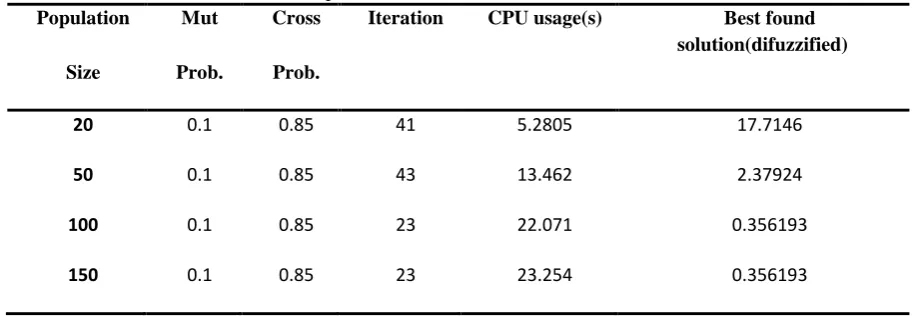
In spite of this high performance in reducing computational time, there is an essential parameter tuning to make best found solution as near as it can be to exact solution (i.e. might not be itself). Table 6shows some effect of changing parameters on average CPU times and the best found solution for 50 jobs instance.

Table 6. Some effect of GA parameter on CPU time and found solution (TF=0.2, DDR=0.4)

In the above table, it could be seen some effects of changing GA parameters on its ability to searching the solution space. Therefore, a comprehensive parameter tuning for hybrid method proves its significance.

4. Hybridization

As it has been said before, GA and DP could be hybrid to achieve advantages of both methods. DP could gain an exact solution but for large instances computational time is appalling, in other hand GA arrive in convergence soon but found solution couldn’t guarantee best possible solution, then if these

Population

Size

Mut

Prob.

Cross

Prob.

Iteration CPU usage(s) Best found

solution(difuzzified)

20 0.1 0.85 41 5.2805 17.7146

50 0.1 0.85 43 13.462 2.37924

100 0.1 0.85 23 22.071 0.356193

methods are combined, an approximation method to deal with these kind of problems appears. Now it illustrates that how it can be possible to launch our method. DP operates as a mother function and recursive manner, and GA plays sub-function role. Suppose ‘n’ jobs must be scheduled, the DP will be called and GA as sub-function finds best searched answer, then method keep last job in memory and apply GA for rest of unscheduled jobs in iterative manner. Some cooling schedule must happen i.e., population size for any recur should be adjusted. In Algorithm 3,pseudo-code of algorithm could be seen.

In each recur keeping the job as scheduled task could be done by two kinds. We can keep first job and then apply GA for rest of them, or put last scheduled job in long term memory and then give rest of unscheduled job to GA. Population size and iteration cooling schedule is strongly related to size of problem and computational limit. GA itself has some techniques that change performance of algorithm such as how to select crossover, way of crossing over etc. cooling schedule can be done in linear state or non-linear one. For making more concentration on the new introduced method let take some assumption:

1- Selecting Parent: tournament 2- Crossing over: one point break 3- Pm and Pc are fix During DP recurs

In Table 8 a comparison between this method and some existing methods for several instances has been drawn into, it may considerable that both under comparison method have been proposed in crisp mode, and authors developed them to be comparable with ours. In Tables 7.1 and Table 7.2 (next two pages) cooling schedule function for population size at each recurs is defined as following:

)

1 1 ( )

(

    

x x m x f

y . (8)

Where, ‘m’ is population size of first recur, and ‘x’is unscheduled jobs number. However, a convenient cooling function could be applied for iteration numbers in each recur, because of existing an un-improved constraint in GA itself, author has preferred to relax cooling function for it. According to the above hypothesis our method can be launched.

Algorithm 3. Pseudo-code of hybrid DP with GA Problem initializing: (S= {1, 2,…, n})

T=processing times; D=Due date; W=jobs weight; Pm=mutation probability; Pc=crossover probability;

Function DP_GA (S,T,D,W,Popsize,Pm,Pc,iter) If (|S|>1)

S=GA (T,D,W,Popsize,Pm,Pc,iter)

S=S\S (last index);

Popsize,iteration=cooling;

DP_GA (S,T,D,W,Popsize,Pm,Pc,iter) Else return(S)

End.

Table 7.1 Result of the method and comparison on some recently produced methods (10 jobs instance have been randomly produced, Population size=50, max-iteration=100, Pm=0.1, Pc=0.85)

TF DDR

Ours

Panneerselvam’s

method

Yoon & Lee’s

Third heuristics

CPU

time

Best found

Obj.

(defuzzified)

CPU

time

found

Objective

(defuzzified)

CPU

time

found

Objective

(defuzzified)

0.2 0.2 8.650509 2.2911 0.020105 14.7859 0.048330 10.1283

0.4 8.243301 1.2195 0.008879 6.6096 0.018795 2.6857

0.6 8.115593 5.1514 0.003777 5.5957 0.010566 5.2636

0.8 8.685870 0 0.003938 5.3340 0.009118 5.0962

1 7.994222 0 0.003748 2.8490 0.011746 1.1886

0.4 0.2 8.794313 10.0177 0.003712 28.3740 0.007750 12.6672

0.4 8.666179 6.1498 0.004233 20.4685 0.011633 6.9719 0.6 10.352173 17.2193 0.003998 43.4039 0.007913 22.7295 0.8 10.292223 6.2413 0.004832 8.1556 0.011564 7.2007

1 10.431836 9.5058 0.003948 30.2888 0.009694 25.2480

0.6 0.2 10.430979 21.7811 0.003796 40.4910 0.011509 27.0675

0.4 11.044465 39.2408 0.003911 81.3758 0.007932 54.6326 0.6 47.2113 10.753702 0.005395 92.5669 0.011746 71.2444 0.8 10.143664 26.0233 0.004224 46.0670 0.007568 39.0497

1 9.254881 18.2142 0.003961 34.5447 0.010416 18.2142

0.8 0.2 11.288370 107.5272 0.003925 148.7824 0.007585 112.7570

0.4 10.231764 64.3247 0.003749 78.2085 0.011800 70.6959

0.6 10.267246 133.0812 0.005441 172.2154 0.007168 142.2375 0.8 10.675864 32.5063 0.003991 83.5434 0.009021 67.3461

1 10.953565 25.4948 0.003480 35.0324 0.008395 33.5310

1 0.2 9.914266 134.9996 0.003257 141.5064 0.009044 134.9996

0.4 11.288335 157.8895 0.002956 181.2881 0.011774 157.8895

0.6 10.405813 134.9299 0.003738 194.6648 0.007556 138.5204 0.8 10.241077 143.0189 0.005021 185.6000 0.009559 154.1998 1 10.802312 59.2854 0.003714 106.2140 0.012424 72.9536

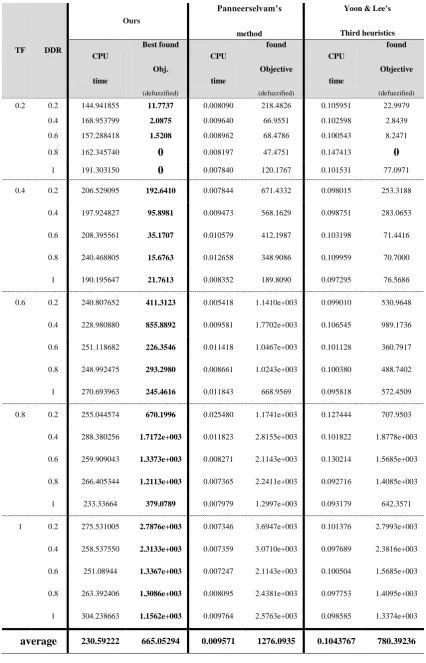
Table 7.2 Results of the method and comparison on some recently produced methods

TF DDR

Ours

Panneerselvam’s

method

Yoon & Lee’s

Third heuristics

CPU

time

Best found

Obj.

(defuzzified)

CPU

time

found

Objective

(defuzzified)

CPU

time

found

Objective

(defuzzified)

0.2 0.2 144.941855 11.7737 0.008090 218.4826 0.105951 22.9979 0.4 168.953799 2.0875 0.009640 66.9551 0.102598 2.8439 0.6 157.288418 1.5208 0.008962 68.4786 0.100543 8.2471

0.8 162.345740 ₀ 0.008197 47.4751 0.147413 ₀

1 191.303150 ₀ 0.007840 120.1767 0.101531 77.0971

0.4 0.2 206.529095 192.6410 0.007844 671.4332 0.098015 253.3188 0.4 197.924827 95.8981 0.009473 568.1629 0.098751 283.0653 0.6 208.395561 35.1707 0.010579 412.1987 0.103198 71.4416 0.8 240.468805 15.6763 0.012658 348.9086 0.109959 70.7000 1 190.195647 21.7613 0.008352 189.8090 0.097295 76.5686 0.6 0.2 240.807652 411.3123 0.005418 1.1410e+003 0.099010 530.9648

0.4 228.980880 855.8892 0.009581 1.7702e+003 0.106545 989.1736 0.6 251.118682 226.3546 0.011418 1.0467e+003 0.101128 360.7917 0.8 248.992475 293.2980 0.008661 1.0243e+003 0.100380 488.7402 1 270.693963 245.4616 0.011843 668.9569 0.095818 572.4509 0.8 0.2 255.044574 670.1996 0.025480 1.1741e+003 0.127444 707.9503 0.4 288.380256 1.7172e+003 0.011823 2.8155e+003 0.101822 1.8778e+003 0.6 259.909043 1.3373e+003 0.008271 2.1143e+003 0.130214 1.5685e+003 0.8 266.405344 1.2113e+003 0.007365 2.2411e+003 0.092716 1.4085e+003 1 233.33664 379.0789 0.007979 1.2997e+003 0.093179 642.3571 1 0.2 275.531005 2.7876e+003 0.007346 3.6947e+003 0.101376 2.7993e+003

0.4 258.537550 2.3133e+003 0.007359 3.0710e+003 0.097689 2.3816e+003 0.6 251.08944 1.3367e+003 0.007247 2.1143e+003 0.100504 1.5685e+003 0.8 263.392406 1.3086e+003 0.008095 2.4381e+003 0.097753 1.4095e+003 1 304.238663 1.1562e+003 0.009764 2.5763e+003 0.098585 1.3374e+003

There is another aspect that in each recur first job in sequence could be kept (forward recurring). However, as it can be manifestly seen that keeping first job of solution in any recur will effect on due dates in next recurs.(Some accumulation happens because omitted or final scheduled jobs processing time summation determines when next recur must count its tardiness, for solving that situation summation of final scheduled jobs must be deducted from due date vector). In Tables 8 and 9, an analysis has been held, between forward and backward recurring. During this comparison wisely all

of parameters have been taken fixed to show only the effect of forward or backward method. A considerable analysis has been revealed that can be conclude, proposed method indicate better solution, however Yoon and Lee’s method can solve the problem like ours, but it happens so rarely. Not only our method outperforms other introduced method, its reduction on best found answer is noticeable (sometimes more than 700% better performance!), that yield proposed method worthy to be noticed. Introduced method work independently of rang and tightness of due dates and it make our method prominent. In Table 7.1for verity of TF and DDR the method has been tested and result was impressive. In Table 7.2,same work has done for large instance to examine methods performance in bigger solution space. In this situation proposed method exceeds others too. However, computational times are greater than two others, But decreasing in found solution could satisfy this accumulation on CPU usage. Even it can be seen that in average, there is a wide fraction between answers of compared methods and ours. Moreover, for large instances ability of proposed method stables through more cost of computational time.

Table 8. A comparison between forward and backward recurring in Hybrid method. (TF=0.2, DDR=0.4)

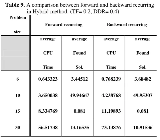
According to two recent tables Table 8 and Table 9, these two aspects are almost equal, but as it can be seen, in general, forward recurring operates faster than other which is because of updating accumulation start time updates, and in searching solution space they are as same as each other however due to GA being probable based, there is some little differences at some cases in e.g. average of 10 jobs problem forward recurring problem backward recurring performed better. So due to importance of computational time, forward recurring is preferred for continuing sessions.

Problem

size

Forward recurring Backward recurring

CPU

Time

Best

Found

Sol.

CPU

Time

Best

Found

Sol.

6 0.965885 3.1272 1.210838 3.1272

10 3.479816 49.5328 4.067849 49.5328

15 8.131612 0.081 10.59722 0.081

30 61.92401 8.5012 72.63574 8.5012

5. Parameter tuning

After seeing a comprehensive analysis on introduced method among some other method, and comparison between two method aspects, there exist many effective factors that had better to be tuned since depth understanding is essential. There are several methods such as cooling function, GA operators’ probability and so on.

Several cooling functions for number of iteration and population size as linear or nonlinear function could be utilized. Some of them exist here:

i. f(x)ax 0a1.

ii. )

1 1 ( )

(

   

k k m k

f .

iii. _f(x)_m(1_exp(_{6x/n)) x}₀. iv. f(x)2xarctg(2nx)/



(9)

Where, ‘x’ is current population size in current recur, ‘m’ is initial population size, ‘k’ is number of

unscheduled job in each recurs, and finally ‘n’ is problem size. In addition, there might be lots of more

convenient cooling functions that were out of authors’ point of view, and they could be an interesting idea to future research. Table 10introduced functions are testes as cooling function of population size, so it can be determined the effect of vary cooling function on methods performance.

Table 9. A comparison between forward and backward recurring in Hybrid method. (TF= 0.2, DDR= 0.4)

Problem

size

Forward recurring Backward recurring

average

CPU

Time

average

Found

Sol.

average

CPU

Time

average

Found

Sol.

6 0.643323 3.44512 0.768239 3.68482

10 3.650038 49.94667 4.238768 49.95307

15 8.334769 0.081 11.19893 0.081

30 56.51738 13.16535 73.13876 10.91536

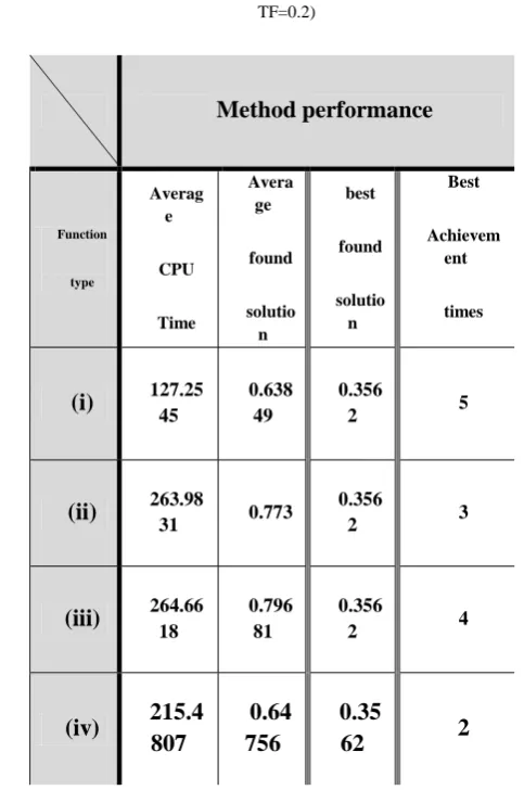
In Table 10,several kind of linear and nonlinear cooling function on population size have been tested. As it can be obvious, function (i) in statement (9) made performance faster, more aggressive, more achievement on best answer. It seems that linear functions are more suitable for cooling.

Also by Table 10,function (iv) performed in average almost equal to (i), but in approximately double computational time and less best solution achievements. Likewise of late table, same analysis could be held for cooling down iteration number at each recurs. However, there is other mechanism that handles cooling automatically. In GA itself one stopping criteria has been put for controlling unimproved iteration, so when the hybrid method runs, naturally at each recurs this condition works and tunes method if convergence has been happened or there is no necessity to continue. Also there is lots of tuning for GA parameters in literature that are also belong to GA special discussion, but here initial population for some instances could be analyzed. In Table 11, some inspection on initial population for several instances by use of (i) function arranged.

Table 10. Testing cooling function on random produced 50 jobs problem

(Pc=0.85, Pm=0.1, initial pop= 100, max-iteration=100 DDR=0.4, TF=0.2)

Method performance

Function

type

Averag e

CPU

Time

Avera ge

found

solutio n

best

found

solutio n

Best

Achievem ent

times

(i) 127.25

45

0.638 49

0.356

2 5

(ii) 263.98

31 0.773

0.356

2 3

(iii) 264.66

18

0.796 81

0.356

2 4

(iv) 215.4

807

0.64 756

0.35

62 2

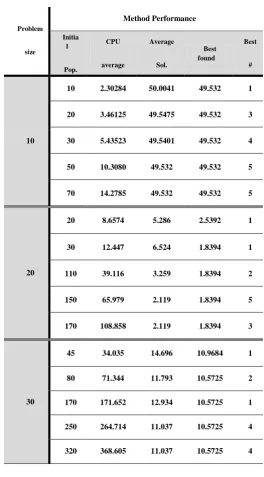
On analyzing Table 11,it could be figured out that increasing in initial population could most of times make last results better; however, it costs much computational time. In addition, there is a case not only increasing initial population didn’t help but also made situation worse (i.e. when problem size was 20, increasing initial population 150 to 170). This observation could be explained by structure of mating pool and selecting parents for being mated, sometimes large population can reduce effect of stronger answer, so it can change final solution a little bite. According to last table, increasing initial population could be ethical till developing in output answer would be gained, and from a threshold increasing only costs more CPU time or sometimes makes output worse; moreover thresholds are considerably related to problem sizes and must be understand practically.

Table 11. Initial population analysis on randomly produced instances (Pc=0.85, Pm=0.1, DDR=0.4, TF=0.2 max-iteration =200)

Problem

size

Method Performance

Initia l

Pop.

CPU

average

Average

Sol.

Best found

Best

#

10

10 2.30284 50.0041 49.532 1

20 3.46125 49.5475 49.532 3

30 5.43523 49.5401 49.532 4

50 10.3080 49.532 49.532 5

70 14.2785 49.532 49.532 5

20

20 8.6574 5.286 2.5392 1

30 12.447 6.524 1.8394 1

110 39.116 3.259 1.8394 2

150 65.979 2.119 1.8394 5

170 108.858 2.119 1.8394 3

30

45 34.035 14.696 10.9684 1

80 71.344 11.793 10.5725 2

170 171.652 12.934 10.5725 1

250 264.714 11.037 10.5725 4

320 368.605 11.037 10.5725 4

6. Conclusion

DP method are widely used in OP and with combination of fuzzy numbers managers and decision makers can use this advanced method for scheduling situation that data is not crisp. Working with exact algorithm like Fuzzy Dynamic programming to solve scheduling on single machine since time and memory restriction might be impossible or unfavorable, so this article recommends using local search heuristic algorithms as it has been tooled such Genetic Algorithm and progress it in fuzzy Dynamic programming world, DP can reduce search area size in on side level by level in each algorithm recur, then GA can productively search within lower dimension area for obtaining local best solution and after in, DP can concatenate solution in all recurs. So in one side we employ DP to reduce our search area and then tools GA to start a greedy search in it. In addition, obviously hybridized problem solver can operate in its best performance and maintain some local optima, while lower dimension search has been done. By the use of GA on this kind of problem it can be regarded that problem will be solved in much reduced computational time, however gaining exact optimal solution can’t be guaranteed and it can’t work on problems that exact solution are determinant, So we can hybridize these algorithm for use their ability in solving problems. According to DP reduction procedure in search area, back warding & Forwarding manner has been checked and forwarding mode due to its faster and better response is preferable. Our method has been compared with some last introduced methods, and in that case easily could be understood that our method work better, however it computes in much more time and this is about searching solution space in greedy manner. Several analysis were held that revealed linear functions can act out better as cooling function, and there is a problem dependent population size threshold. Finally working with trapezoidal fuzzy numbers and fuzzy due dates (full fuzzy condition), using other heuristics and cooling functions, analyzing cooling function coefficients could be recommended for future researches.

Acknowledgment

The authors greatly appreciate to International Center of Optimization and Decision Making (ODM) for its support.

References

[1] Bellman, R. (2013). Dynamic programming. Courier Corporation.

[2] Ebrahimnejad, A., Nasseri, S. H., Lotfi, F. H., & Soltanifar, M. (2010). A primal-dual method for linear programming problems with fuzzy variables. European Journal of Industrial Engineering, 4(2), 189-209.

[3] Nasseri, S. H., & Ebrahimnejad, A. (2010). A fuzzy primal simplex algorithm and its application for solving flexible linear programming problems. European Journal of Industrial Engineering, 4(3), 372-389.

[4] Mahdavi-Amiri, N., & Nasseri, S. H. (2007). Duality results and a dual simplex method for linear programming problems with trapezoidal fuzzy variables. Fuzzy sets and systems, 158(17), 1961-1978. R.E.

[5] Bellman, R. E., & Zadeh, L. A. (1970). Decision-making in a fuzzy environment. Management science, 17(4), B-141.

[7] Novoa, C., & Storer, R. (2009). An approximate dynamic programming approach for the vehicle routing problem with stochastic demands. European Journal of Operational Research, 196(2), 509-515.

[8] Höfferl, F., & Steinschorn, D. (2009). A dynamic programming extension to the steady state refinery-LP. European Journal of Operational Research, 197(2), 465-474.

[9] Xiong, Y., & Rao, S. S. (2005). A fuzzy dynamic programming approach for the mixed-discrete optimization of mechanical systems. Journal of Mechanical Design, 127(6), 1088-1099.

[10] Trzaskalik, T., & Sitarz, S. (2007). Discrete dynamic programming with outcomes in random variable structures. European Journal of Operational Research, 177(3), 1535-1548.

[11] Pal, B. B., & Moitra, B. N. (2003). A goal programming procedure for solving problems with multiple fuzzy goals using dynamic programming. European Journal of Operational Research, 144(3), 480-491.

[12] Safaei, N., Saidi-Mehrabad, M., Tavakkoli-Moghaddam, R., & Sassani, F. (2008). A fuzzy programming approach for a cell formation problem with dynamic and uncertain conditions. Fuzzy Sets and Systems, 159(2), 215-236.

[13] Holland, J. H. (1992). Adaptation in natural and artificial systems: an introductory analysis with applications to biology, control, and artificial intelligence. MIT press.

[14] Lee, K. Y., & El-Sharkawi, M. A. (Eds.). (2008). Modern heuristic optimization techniques: theory and applications to power systems (Vol. 39). John Wiley & Sons.

[15] Eberhart, R. C., & Shi, Y. (2007). Computational intelligence. Morgan Kaufmann.

[16] Malandraki, C., & Dial, R. B. (1996). A restricted dynamic programming heuristic algorithm for the time dependent traveling salesman problem. European Journal of Operational Research, 90(1), 45-55.

[17] Park, Y. M., Park, J. B., & Won, J. R. (1998). A hybrid genetic algorithm/dynamic programming approach to optimal long-term generation expansion planning. International Journal of Electrical Power & Energy Systems, 20(4), 295-303.

[18] Patra, S., Goswami, S. K., & Goswami, B. (2009). Fuzzy and simulated annealing based dynamic programming for the unit commitment problem. Expert Systems with Applications, 36(3), 5081-5086. [19] Tang, L., & Ren, H. (2010). Modelling and a segmented dynamic programming-based heuristic approach for the slab stack shuffling problem. Computers & Operations Research, 37(2), 368-375. [20] Ibaraki, T., & Nakamura, Y. (1994). A dynamic programming method for single machine

scheduling. European Journal of Operational Research, 76(1), 72-82.

[21] Li, D. C., & Li, T. Y. (1988). An algorithm for sequencing jobs to minimize total tardiness. Journal of the Chinese Institute of Engineers, 11(6), 653-659.

[22] Jinjiang, Y. U. A. N. (1992). The NP-hardness of the single machine common due date weighted tardiness problem, Syst. Sci. Math. Sci,5, 328–333.

[23] Tuong, N. H., Soukhal, A., & Billaut, J. C. (2010). A new dynamic programming formulation for scheduling independent tasks with common due date on parallel machines. European Journal of Operational Research, 202(3), 646-653.

[24] Bosio, A., & Righini, G. (2009). A dynamic programming algorithm for the single-machine scheduling problem with release dates and deteriorating processing times. Mathematical methods of operations research, 69(2), 271.

[25] Koulamas, C. (2009). A faster fully polynomial approximation scheme for the single-machine total tardiness problem. European Journal of Operational Research, 193(2), 637-638.

[26] Kacem, I. (2010). Fully polynomial time approximation scheme for the total weighted tardiness minimization with a common due date. Discrete Applied Mathematics, 158(9), 1035-1040.

[27] Kacem, I. (2010). Fully polynomial time approximation scheme for the total weighted tardiness minimization with a common due date. Discrete Applied Mathematics, 158(9), 1035-1040.

[28] Khorshidian, H., Javadian, N., Zandieh, M., Rezaeian, J., & Rahmani, K. (2011). A genetic algorithm for JIT single machine scheduling with preemption and machine idle time. Expert systems with applications, 38(7), 7911-7918.

[29] Bilge, Ü., Kurtulan, M., & Kıraç, F. (2007). A tabu search algorithm for the single machine total weighted tardiness problem. European Journal of Operational Research, 176(3), 1423-1435. [30] Xu, K., Feng, Z., & Jun, K. (2010). A tabu-search algorithm for scheduling jobs with controllable

processing times on a single machine to meet due-dates. Computers & Operations Research, 37(11), 1924-1938.

[32] Liu, L., & Zhou, H. (2013). Hybridization of harmony search with variable neighborhood search for restrictive single-machine earliness/tardiness problem. Information Sciences, 226, 68-92.

[33] Altunc, A. B. C., & Keha, A. B. (2009). Interval-indexed formulation based heuristics for single machine total weighted tardiness problem. Computers & Operations Research, 36(6), 2122-2131. [34] Lee, J. Y., & Kim, Y. D. (2012). Minimizing the number of tardy jobs in a single-machine scheduling

problem with periodic maintenance. Computers & Operations Research, 39(9), 2196-2205. [35] Panneerselvam, R. (2006). Simple heuristic to minimize total tardiness in a single machine scheduling

problem. The International Journal of Advanced Manufacturing Technology, 30(7), 722-726. [36] Yoon, S. H., & Lee, I. S. (2011). New constructive heuristics for the total weighted tardiness

problem. Journal of the Operational Research Society, 62(1), 232-237.

[37] Yager, R. R. (1981). A procedure for ordering fuzzy subsets of the unit interval. Information sciences, 24(2), 143-161.