Published online November 19, 2014 (http://www.sciencepublishinggroup.com/j/ajaf) doi: 10.11648/j.ajaf.s.2014020601.11
ISSN: 2330-8583 (Print); ISSN: 2330-8591 (Online)
Modification, calibration and validation of APSIM to suit
maize (
Zeamays L.
) production system: A case of Nkango
Irrigation Scheme in Malawi
John Mthandi
1, *, Fredrick C. Kahimba
1, Andrew K. P. R. Tarimo
1, Baandah. A. Salim
1,
Max W. Lowole
21
Department of Agri. Eng. and Land Planning, Sokoine University of Agriculture, Morogoro, Tanzania
2
Department of Crop Science, Bunda College of Agriculture, Lilongwe, Malawi
Email address:
[email protected] (Mthandi J.)
To cite this article:
John Mthandi, Fredrick C. Kahimba, Andrew K. P. R. Tarimo, Baandah. A. Salim, Max W. Lowole. Modification, Calibration and Validation of APSIM to Suit Maize (Zeamays L.) Production System: A Case of Nkango Irrigation Scheme in Malawi. American Journal of Agriculture and Forestry. Special Issue: Agriculture Ecosystem and Environment. Vol. 2, No. 6-1, 2014, pp. 1-11. doi: 10.11648/j.ajaf.s.2014020601.11
Abstract:
Nitrogen (N) is the most important nutrient in maize production and its availability can affect the production potential of maize. Availability of nitrogen in soil largely varies with place and time. Models are some of practical methods used to evaluate and monitor availability and impact of nitrogen on maize production; APSIM is one of such models. APSIM has several modules that have different functionalities and one of such modules is SoilWat module. The study modified SoilWat module by incorporating Nitrogen Distribution model. Trial and error method was used in the calibration of the nitrogen distribution model that was incorporated in the APSIM model as subroutine. The initial values of nitrogen distribution were obtained from literature and these values formed the basis for development of the model. After development of model using parameters obtained from literature review, field experiment was conducted to collect data to be used in redefining the model. The simulated nitrogen distribution was compared with values obtained from the field experiment and their mean differences were initially high but the process was repeated until the mean difference was small. In field experiment, the study had two factor, each with four regimes. The Triscan Sensor (EnviroScan, Sentek Pty Ltd, Stepney, Australia) was used to measure total nitrogen concentration at lateral distances and vertical depths. Primary soil samples were collected and analysed at Bunda College Laboratory. The study inferred that Soil water percolates down to underlying layer only when proceeded layers are satisfied i.e. has reached its field capacity, above which excess water is left free to percolates down the soil profile. Before water arriving in last layer it had to satisfy the above-lying soil profiles. The study has shown that increase of nitrogen contents in underlying layers corresponds with decrease of the same in top layers due to advection movement. Consequently, the increases of soil water in a specific layer correspond to decrease of nitrogen content in that particular layer. The study has shown that APSIM under predicted during the latter stage of the maize growing season and over predicted in the early stage of the growing season, and it overestimates soil water contents in soil profile.Keyword:
APSIM, Soil Water Content, Nitrogen Concentration, Maize1. Introduction
Nitrogen (N) is the most limiting factor in maize production [1]. Increasing N fertilization increases corn grain yield [2,3] and increasing soil moisture enhances maize yield response to N fertilization, especially when high N rates are applied [4,5]. The requirement of nitrogen fertilizer by maize varied temporally and spatially among and within seasons [6]. N fertilizer management practices that do not accommodate
2 John Mthandi et al.: Modification, Calibration and Validation of APSIM to Suit Maize ( A Case of Nkango Irrigation Scheme
required, and too variable to be practical at the farm scale Modeling is one approach used to address the increasing need of understanding the implications of management decisions on N cycling and leaching. The models are built using set of equations that governs the transport of nutrients including N in soil. N movement in soil can
described by the phenomenon of solutes transport in soil. The N movement in soil is predominantly by three basic mechanisms of solute transport namely Advection, diffusion, and dispersion [9, 10, 11]. Based on these three basic mechanisms several models have been developed to infer behaviour of N in the soil and some of these models are as follows: LEACHMN [12], RZWQM [13,
HYDRUS program [16], and APSIM [17].
The Agricultural Production Systems sIMulator (APSIM) is a multi-purpose and comprehensive model developed as a tool for exploring crop management strategies that can improve the economics of agricultural production systems and the consequences of the soil resources and environment [18]. APSIM is a modeling framework that
coupling of various one-dimensional models from separate research efforts into a single simulation. It is used to study interactions between plants, soil, water, and nutrients The APSIM is a centralized engine into which different modules that enable the simulation of systems covering a range of plant, animal, soil, climate and management interactions could be connected.
Figure 1 indicates different modules of APSIM, which have different functionalities and can be used depending on type of decisions to be used. Each module provides a small piece of simulation functionality with the ‘engine’ coordinating the flow of data/variables between the modules. The SoilN module describes the dynamics and processes of carbon and nitrogen in soil, and the SoilWater module
Fig. 2. Flow diagram of communication between SoilWat and other APSIM modules (Source: www.apsim.i The SoilWat module do not consider the spreading pattern
of nitrogen and water in both lateral and vertical dimensions
: Modification, Calibration and Validation of APSIM to Suit Maize (Zeamays L.
A Case of Nkango Irrigation Scheme in Malawi
required, and too variable to be practical at the farm scale [8]. pproach used to address the increasing need of understanding the implications of management decisions on N cycling and leaching. The models are built using set of equations that governs the transport of nutrients N movement in soil can therefore be described by the phenomenon of solutes transport in soil. The N movement in soil is predominantly by three basic mechanisms of solute transport namely Advection, diffusion, . Based on these three basic eral models have been developed to infer behaviour of N in the soil and some of these models are as 14], NLEAP [15], .
The Agricultural Production Systems sIMulator (APSIM) rpose and comprehensive model developed as a tool for exploring crop management strategies that can improve the economics of agricultural production systems and the consequences of the soil resources and environment APSIM is a modeling framework that allows the dimensional models from separate research efforts into a single simulation. It is used to study interactions between plants, soil, water, and nutrients [17]. The APSIM is a centralized engine into which different that enable the simulation of systems covering a range of plant, animal, soil, climate and management
Figure 1 indicates different modules of APSIM, which have different functionalities and can be used depending on f decisions to be used. Each module provides a small piece of simulation functionality with the ‘engine’ coordinating the flow of data/variables between the modules. The SoilN module describes the dynamics and processes of SoilWater module
account for solute movement in the soil
Fig. 1. Different modules of APSIM (Source: www.apsim.ingo) 1.1. Solutes Movement in the Soil
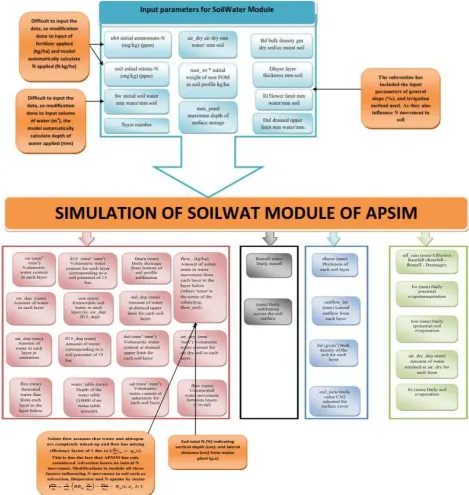
A SoilWat module calculates the redistribution of water and solutes throughout the soil profile using separate algorithms for saturated or unsaturated flow. The redistribution of solutes, such as nitrate- and urea-N, is carried out in this module. The algorithm assumes that all water and solutes entering or leaving a layer is completely mixed and flow has efficiency factors of 1.0 meaning that solute movement can simply be calculated as the product of the water flow and the solute concentration in that water
SoilWat module is an integral module of APSIM; it links other modules for APSIM to simulate properly (Figure 2). The SoilWater module is responsible for movement of water, solutes and heat from one place to the other within the system. The SoilWat module has
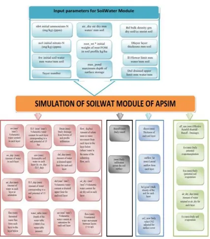
that perform various functionalities within the module as indicated in figure 3 below.
Flow diagram of communication between SoilWat and other APSIM modules (Source: www.apsim.i
do not consider the spreading pattern of nitrogen and water in both lateral and vertical dimensions
to establish the amount of nitrogen deposited in the rooting zone. [19] reported APSIM models do not c
Zeamays L.) Production System:
account for solute movement in the soil [18].
Different modules of APSIM (Source: www.apsim.ingo)
in the SoilWat Module
module calculates the redistribution of water and solutes throughout the soil profile using separate algorithms for saturated or unsaturated flow. The redistribution of solutes, N, is carried out in this module. The mes that all water and solutes entering or leaving a layer is completely mixed and flow has mixing meaning that solute movement can simply be calculated as the product of the water flow and the solute concentration in that water [18].
SoilWat module is an integral module of APSIM; it links other modules for APSIM to simulate properly (Figure 2). The SoilWater module is responsible for movement of water, solutes and heat from one place to the other within the odule has five different Subroutines that perform various functionalities within the module as
Flow diagram of communication between SoilWat and other APSIM modules (Source: www.apsim.ingo)
flow or horizontal heterogeneity. APSIM only account for the nitrogen content entering and leaving each layer but not distribution pattern of nitrogen in each layer. However, [20] reported that previous tests of APSIM have shown that modifications to APSIM‘s parameters that control the extent of mixing of percolating water may be required to improve estimates of the movement of N in soil. This paper undertakes modification and calibration of solute flux subroutine of SoilWater module in the ASPIM model so as to improve prediction capacity of model on the N movement in soil in Malawi. Figure 4 below shows the flow chart of SoilWat module of APSIM. It shows the input parameters, the processes and output parameters.
Fig. 3. Subroutine structure of SoilWat module in APSIM
4 John Mthandi et al.: Modification, Calibration and Validation of APSIM to Suit Maize (Zeamays L.) Production System: A Case of Nkango Irrigation Scheme in Malawi
2. Materials and Methods
2.1. Calibration of the Nitrogen Distribution Subroutine
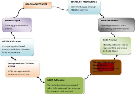
Trial and error method was used in the calibration of the nitrogen distribution model that was incorporated in the APSIM model as subroutine. Trial and error is a method of solving problems and is characterised by repeated, varied attempts which are continued until success. [21] reported that trial and error method involves assigning an initial value usually from values found in literature or field experimental
data relating to the parameter to be estimated by calibration. The initial values of nitrogen distribution in the soil were obtained from literature and these values formed the basis for development of the model. After development of model using parameters obtained from literature review, field experiment was conducted to collect data to be used in redefining the model. The simulated nitrogen distribution was compared with values obtained from the field experiment and their mean differences were initially high. The process was repeated until the mean difference was small.
Fig. 5. Model development process 2.2. Field Experiments
The field experiment was carried out at Nkango Irrigation Scheme in Kasungu district, Malawi. Data were collected at growing seasons of 1st June to 8th September, 2012; and 10st September to 5th December, 2012. The scheme is situated at Latitude 12035’ South and Longitudes 33031’ East and is at 1186 m above mean sea level. The mean annual rainfall is about 800 mm. The site has coarse sandy loam as the dominant soil type. The study plots were 5 X 5 m in size and ridges were spaced at 75 cm apart. The distance between plot to plot were 2 metre for avoiding ‘sharing’ of responses, water and nitrogen (edge effects). Three maize seeds of hybrid maize (SC 407) were planted per hole at spacing of 25 cm. They were later on thinned to one seed per station 7 days after germination.
The trials consisted of factorial arrangement in a Randomised Complete Block Design (RCBD). The factors
were water and nitrogen and both at four levels. Water had four application regimes viz farmers’ practice regime; full (100%) water requirement regime (FWRR) of maize plant; 60% of FWRR and 40% of FWRR. A full maize water requirement was determined by the procudure described by Allen et al., (1998). Nitrogen also had four application regimes i.e. the typical nitrogen application rate in the area (TNPRA) of 92 kg N/ha was used as a basis to determine other dosage levels in the study[22]. The nitrogen dosage levels were TNPRA, 92 kg N/ha; 125% of TNPRA, 115 kg N/ha; 75% of TNPRA, 69 kg N/ha and 50% of TNPRA, 46 kg N/ha. The fertlizer was applied two times, basal and top dressings, 21 and 51 days after planting, respectively.
nitrogen concentration at lateral distances. The measurement of the sensor are in Volumetric Ion Concentration (VIC), but using standazation equation the concentration of total nitrogen on each point was known. The lateral distances at which measurements were taken were as follows: at point of application (represented by 0 cm), at 5 cm away from the plant (represented by -5 cm), at 5 cm towards the plant, 10 cm towards the plant (this point was maize planting station), and 15 cm (this point was 5 cm after planting station in the direction opposite from where N was applied). The lateral distances were taken based on spreading and elongation pattern of lateral roots of maize plants.
The lateral reading of nitrogen were respecively taken at
five soil depths of 20, 40, 60, 80, and 100 cm. The soil depths were selected based on maize roots growth habits which extend down to 100 cm [23]. Confirmation of data was done through analyising soil samples collected from the respective points. The soil profile was dug to a depth of 120 cm using soil auger. Soil samples were collected from the lateral points for laborotary analysis.
Primary soil samples were collected and analysed at Bunda College Laboratory to know the values of wilting point or Lower Limit of soil water content at 15 Bar (LL15), Drained Upper Limit of soil water content (DUL) or Field Capacity, and Saturated soil water content (SAT). The hydraulic conductivities of soil were from the soil literature review.
6 John Mthandi et al.: Modification, Calibration and Validation of APSIM to Suit Maize (Zeamays L.) Production System: A Case of Nkango Irrigation Scheme in Malawi
3. Results and Discussion
3.1. Total Nitrogen Contents in the Soil
Majority of nitrogen available to plants is in the form of inorganic NH4+ and NO3-. Ammonium ions (NH4+) bind to
the soil’s negatively-charged Cation Exchange Complex (CEC), while nitrate ions (NO3-) do not bind to the soil solids
because they carry negative charges. Since none of the nitrate is adsorbed to soil particles it is abundant in the soil water and the movement of the nitrate to the root rarely limits its uptake.
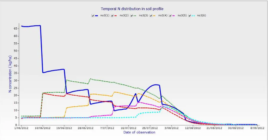
Figure 7 shows the simulated temporal distribution of nitrogen within the soil profile of 100FWRR plot which received TNPRA. The no3(1) shows the concentration of nitrogen in the first layer (0-10 cm), no3(2) shows the nitrogen concentration in the second layer (10-20 cm), the nitrogen concentration in third layer (20-40 cm) is being represented by no3(3). The figure indicates that on 1/06/2012 the nitrogen concentration in first layer was above 65 N kg/ha while the concentration in underlying layers were all around 5 N kg/ha. This is because on 1/06/2012, NPK
(23:21:0+4s) fertilizer was basal dressed and hence high concentration of N at the point of application. The other underlying layers still had the residual nitrogen concentration which was 5 N kg/ha. On 10/06/2012, N concentration second layer (10-20 cm) and third layer (20-40 cm) had increased from 5 N kg/ha to above 20 N kg/ha, while that of first layer [no3 (1)] had reduced from above 65 N kg/ha to about 35 N kg/ha. This change of N concentrations can be explained by movement of water which carried N solute down to underlying (second and third) layers. This can further be validated by trend of soil water movement in figure (12) below. Another line of interest is no3 (6) which is N concentration in last layer (80-100 cm), figure 7 shows that N concentration remained relatively constant until after 16/07/2012 indicating that soil water arrived to this layer on this particular day. This can as well be confirmed by the trends of water movement in figure (12) below, which also indicates that soil water arrived in the last layer after six irrigation events. The increase of N concentration on 16/07/2012 is due to second application (top dressing) of urea fertilizer, which was applied 45 days after planting.
Fig. 7. Temporal distribution of nitrogen in 100FWRR plot which received TNPRA.
Fig. 8. Comparison between observed and simulated N concentration at top layer (0-20 cm).
N concentration in first layer. The APSIM under predicted during the latter stage of the maize growing season and over predicted in the early stage of the growing season. This therefore suggests that APSIM does not perfectly predict concentration of nitrogen. [20] also reported that APSIM simulations over estimate the soil solution nitrate concentration.
Fig. 9. Comparison between observed and simulated N concentration at bottom layer (80-100 cm).
Figure 9 shows changes in N concentrations within the bottom layer (80-100 cm) of plot that received TNPRA. From 1/06/2012 to 30/06/2012 the change of N concentrations between simulated and observed data is small. The trend indicates that in simulated data, there was no addition of new concentration of nitrogen while in observed data; there was a small addition of N concentrations. From 30/07/2012, the N concentration from observed data is higher than from simulated data indicating that APSIM is underestimating the N concentration in last layer.
3.2. Soil Water Contents in the Soil
In this section of the paper, soil water contents from simulated and observed data have been presented and explained. Unless specified the unit of soil water content in the soil is given as millimeter of water in millimeter of soil depth (mm/mm). Figure 10 presents the amount of water applied in the plot from which proceeding figures of soil water contents have been taken and discussed.
Fig. 10. Amount of water applied in 100FWRR plot which received TNPRA. Figure 10 shows the time of water application and amount of water applied in a plot that received full water requirement regime presented as 100FWRR. This plot also received 92 N kg/ha of nitrogen presented as Typical Nitrogen Application Regime in the Area (TNPA). Amount of water applied in each irrigation event was 84 mm of water and was applied after every 10 days. The first application was done on 1st June 2012 and the last application event was done on 8th September, 2012.
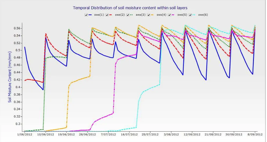
Fig. 11. Simulated soil moisture distribution in the soil profile. Figure 11 shows soil water distribution through the soil
profile as simulated by the by APSIM from 100FWRR plot which received TNPRA. From figure 12 it shows that soil
8 John Mthandi et al.: Modification, Calibration and Validation of APSIM to Suit Maize (Zeamays L.) Production System: A Case of Nkango Irrigation Scheme in Malawi
mm/mm before next irrigation on 10th June, 2012. This sharp declined can be explained as due to massive soil water loss through evaporation as during this time, crop cover had not fully covered the soil to reduce soil evaporation. From 19/06/2012, sws (1) line has its difference of soil water contents between when water was applied to the last day before next application reduced i.e. it is more flatter than compared to before 19/06/2012 and after 3/08/2012. The trend can be explained by crop cover which fully covered the soil and hence reduce soil evaporation. Another trend of interest is sws (6) line which is last section of soil profile (80-100cm), the line started to peak on 7/07/2012 which is almost 37days after first water application i.e. after 5 water applications. From 1/06/2012, the soil water content was stagnant at 0.28 mm/mm. Soil water percolates through soil profile only when proceeded soil is satisfied i.e. has reached its field capacity, above which excess water is left free to percolates down the soil profile. Before water arriving in last layer it had to satisfy the above-lying soil profiles. However, when water had reached in this layer, the soil water lose was small and this is the reason why the sws (6) line is flatter than compared to all other soil water lines. This observation is similar to that of many literatures which explain that fluctuations of soil water contents in bottom layers of soil profiles are small compared to top layer. Another observation from the graph is that even during irrigation time, soil water content never exceeded 0.56 mm/mm indicating that the saturation point of this soil is 0.56mm/mm. figures 12 and 13 below are comparing differences of simulated soil water contents to the observed soil water contents within the top layer (0-20cm) and bottom layer (80-100cm).
Fig. 12. Comparison of simulated and observed soil water distribution within top layer 0-20cm
Figure 12 shows the comparison between simulated and observed soil water distribution within the first layer (0-20 cm) of 100FWRR plot which received TNPRA. The figure 11 indicates that observed soil water contents were far less compared with simulated soil water contents. The soil water contents from observed graph line indicates that were within 0.14 to below 0.28 mm/mm of soil, while soil water contents from simulated graph line were within the range of 0.51 to 0.558 mm/mm of soil. Figure 12 shows that APSIM had overestimated soil water contents of top layer in 100FWRR plot of TNPRA.
Figure 13 shows soil water distribution within 80-100 cm layer over the growing season in 100FWRR plot which received TNPRA. From figure 13 it can be seen that observed graph line is below simulated graph line meaning that observed soil water contents were less to that of simulated soil water contents. However, both graph lines in figure 13 are showing similar trend in the way they are increasing and decreasing.
Fig. 13. Comparison of simulated and observed soil water distribution within bottom layer (80-100cm).
3.3. Relationship of Soil Water and Nitrogen Content in Soil
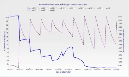
Fig. 14. Showing relationship of soil water and nitrogen content in top layer (0-10cm) of 100FWRR plot which received TNPRA
Fig. 15. Showing relationship of soil water and nitrogen content in third layer (20-80cm) of 100FWRR plot which received TNPRA. Figure 15 indicates an increase in soil water and nitrogen
contents from below 0.3 mm/mm and over 5 N kg/ha on 01/06/2012 to over 0.48 mm/mm and over 20 N kg/ha on 10/06/2012 respectively. The increase in soil water and nitrogen content in this layer corresponds with decrease in nitrogen content in top layer as shown in figure 14 above. The other interesting observation in figure 15 is the soil water and nitrogen contents trends from 10/06/2012 to 07/07/2012. The trend appears to show the similar pattern of increase and
10 John Mthandi et al.: Modification, Calibration and Validation of APSIM to Suit Maize (Zeamays L.) Production System: A Case of Nkango Irrigation Scheme in Malawi
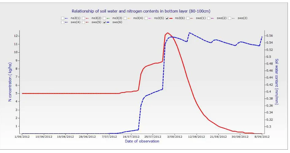
Fig. 16. Showing relationship of soil water and nitrogen content in third layer (80- 100cm) of 100FWRR plot which received TNPRA. From 01/06to 16/07/2012 in figure 16, N concentration
remained the same on about 5 N kg/ha, which increased to about 8 N kg/ha on 25/07/2012 and subsequently increased to its highest concentration of about 11 N kg/ha before it started to decline on 03/08/2012 to almost 0 on 08/09/2012. Soil water content increased in similar fashion from below 0.3 mm/mm to 0.38 mm/mm and subsequently to over 0.54 mm/mm in just 10 days from 16/07/2012, despite staying constant on 0 for 46 days from 01/06/2012. The sudden rise of soil water and nitrogen contents in this layer shows that overlying layers had their ‘needs’ satisfied as such additional application of water just moved to this bottom layer without any hindrance (being held by soil particles).
4. Conclusions
The following conclusions have been drawn from the study: Soil water percolates down to underlying layer only when proceeded layers are satisfied i.e. has reached its field capacity, above which excess water is left free to percolates down the soil profile. Before water arriving in last layer it had to satisfy the above-lying soil profiles. This therefore suggests that to avoid deep percolation and losing of nitrogen to layers below maize rootzone, water applied should correspond to the amount of water that can be retained in soil layers of maize rootzone. The study has shown that increase of nitrogen contents in underlying layers corresponds with decrease of the same in top layers due to advection movement. Consequently, the increases of soil water in a specific layer correspond to decrease of nitrogen content in that particular layer. This suggests that to maximise deposition of nitrogen within rooting zone of maize plant, amount of applied water should be reduced after nitrogen application. Movement of nitrogen through soil profile corresponds to amount of water applied. The study has
shown that APSIM under predicted during the latter stage of the maize growing season and over predicted in the early stage of the growing season, and it overestimates soil water contents in soil profile.
References
[1] Uribelarrea, M., Crafts-Brandner, S.J., Below, F.E., 2009. Physiological N response of field-grown maize hybrids (Zea mays L.) with divergent yield potential and grain protein concentration. Plant and Soil, 316, 151-160.
[2] Mullins, G.L., Alley, S.E., Reeves, D.W., 1998. Tropical maize response to nitrogen and starter fertilizer under strip and conventional tillage systems in southern Alabama. Soil Till. Res. 45, 1-15.
[3] Halvorson, A.D., Mosier, A.R., Reule, C.A., Bausch, W.C., 2006. Nitrogen and tillage effects on irrigated continuous corn yields. Agron. J. 98, 63-71.
[4] Eck, H.V., 1984. Irrigated corn yield response to nitrogen and water. Agron. J. 76, 421-428.
[5] Al-Kaisi, M.M., and X. Yin. 2003. Effects of nitrogen rate, irrigation rate, and plant population on corn yield and water use efficiency. Agron. J. 95: 1475 – 1482.
[6] Devienne-Barret, F., Justes, E., Machet, J.M., Mary, B., 2000. Integrated control of nitrate uptake by crop growth rate and soil nitrate availability under field conditions. Ann. Bot. 86, 995-1005.
[7] Russell, A.E., Laird, D.A., Mallarino, A.P., 2006. Nitrogen fertilization and cropping system impacts on soil quality in midwestern mollisols. Soil Sci. Soc. Am. J. 70, 249-255.
[9] Jury, W.A., Gardner, W.R. and Gardner, W.H. 1991. Soil physics. 5th edition. John Wiley and Sons. New York.
[10] Van Genuchten, M.Th., Leij, F.J., Yates, S.R., 1991. The RETC code for quantifying the hydraulic functions of unsaturated soils. USAEPA Rep. 600/2-91/065. R.S. Kerr Environmental Research Laboratory. Ada, OK 74820.
[11] Vitousek, P.M., Hattenschwiler, S., Olander, L. and Allison, S. 2002. Nitrogen and nature. Ambio. 31: 97-101
[12] Hutson, J.L. and Wagenet, R.J. 1993. A pragramatic field scale approach for modelling pesticides. Journal of Environmental Quality 22: 494–499.
[13] Hanson, J.D., Rojas, K.W. and Shaffer, M.J. 1999. Calibrating the root zone water quality model. Agronomy Journal. J. 91:171–177.
[14] Ahuja, L.R., Rojas, K.W., Hanson, J.D., Shaffer, M.J. and Ma L. (eds.). 2000. Root zone water quality model: Modelling management effects on water quality and crop production. Water Resources Publications LLC, Highlands Ranch, Co. 372 pp.
[15] Shaffer, M. J., Halvorson, A. D. and Pierce, F. J. 1991. Nitrate leaching and economic analysis package (NLEAP): Model description and application. Pages 285–322. In R. F. Folet et al. (eds.). Managing nitrogen for groundwater quality and farm profitability. SSSA, Madison WI.
[16] Simunek, J., Sejna, M. and van Genuchten, M.Th. 1999. The HYDRUS-2D software package for simulating two-dimensional movement of water, heat, and multiple solutes in variably saturated media. Version 2.0, IGWMC - TPS - 53,
International Ground Water Modeling Center, Colorado School of Mines, Golden, Colorado, 251pp.
[17] McCown, R.L., Hammer, G.L., Hargreaves, J.N.G., Holzworth, D.P. and Freebairn, D.N. (1996). APSIM: A novel software system for model development, model testing, and simulation in agricultural research. Agricultural Systems 50: 255-271.
[18] Probert, M.E., J.P. Dimes, B.A. Keating, R.C. Dalal, and W.M. Strong. 1998.APSIM’s water and nitrogen molecules and simulation of the dynamics of water and nitrogen in fallow systems. Agricultural systems, 56, 1-28,
[19] Sharp, J.M., Thomas S.M, Brown, H.E. 2011. A validation of APSIM nitrogen balance and leaching predictions. The New Zealand Institute for Plant & Food Research Limited, Private Bag 4704, Christchurch, 8140, New Zealand.
[20] Allen, R.G., L.S. Pereira, D. Raes, and M. Smith. 1998. Crop evapotranspiration. Guidelines for computing crop water requirements. Irrig. And Drainage Paper no. 56.
[21] Salim, B.A. (1999). Modelling and Measurement of Soil Moisture Content Based on a Remote Sensing Method for Application in Semi-Arid Tropics. PhD dissertation. Institut fur Landtechik der Rheinischen Friedrich-Wilhelms-Universitaet Bonn, pp. 148-149.
[22] Ministry of Agriculture and Food Security. (2011). Annual reports and notes. Lilongwe, Malawi.
[23] FOASTAT (2000) Maize.