Published online October 20, 2014 (http://www.sciencepublishinggroup.com/j/ijepe) doi: 10.11648/j.ijepe.20140305.13
ISSN: 2326-957X (Print); ISSN: 2326-960X (Online)
Predicting heat demand for a district heating systems
Krzysztof Wojdyga
Faculty of Environmental Engineering, Warsaw University of Technology, Warsaw, Poland
Email address:
To cite this article:
Krzysztof Wojdyga. Predicting Heat Demand for a District Heating Systems. International Journal of Energy and Power Engineering. Vol. 3, No. 5, 2014, pp. 237-244. doi: 10.11648/j.ijepe.20140305.13
Abstract:
Poland is one of the heaviest users of district heating systems in Europe, and those district heating systems are heated mainly by coal. Sustainable development of district heating systems in Poland including improving quality of environment, economic of heat production and security of heat supply is in close connection with increasing of energy efficiency. Heat production and heat distribution plays important role in national energy balance. Additional increasing of energy efficiency in district heating systems need detail forecasts for future heat consumption in scale of individual district heating system and for systems in whole country. Accurate forecast give possibility for increasing efficiency of heat production, decreasing fuel consumption and connected with it emission decreasing from combustion products to the atmosphere. Heat production efficiency can be optimized through the use of appropriate procedures for running heat sources alongside short-term heat demand forecasting combined with preparation for adjusting heat source work parameters to the predicted heat load for a few hours hence. The artificial neural networks model delivers good forecasting results. The accuracy of the results depends on the kind of network, its architecture, the size and type of input data as well as the forecasting period. Forecasting accuracy within a 3-5% margin of error is sufficient to steer heat source operations. Described forecasting methods can be use as a good tool to regulate district heating networks and heat sources.Keywords:
District Heating Systems, Heat Demand Prediction1. Introduction
In urban areas with high density of demand for heat, the most rational and economical means of heat supply for the inhabitants are district heating systems. Large sources producing heat for heating systems are generally equipped with high-efficiency units, limiting emissions of combustion products into the atmosphere. The emission of pollutants from small, local and dispersed sources consuming inferior fuels is higher in relative terms than from centralized sources. District heating, a very important energy sub-sector for the Polish economy, supplies heat to centralized heating systems which, on average, satisfy 72% of the demand for heat in Polish cities[1]. In the 1990s, Poland embarked on the process of modernizing its heating systems. At that time there was also a reduction in heat demand of over 30% due to the thermomodernization of buildings. The reduction in heat demand was visible despite numerous new recipients joining the system.
Sustainable development of heating systems in Poland is closely connected with further increases in energy efficiency both on the part of recipients and heat producers. The
modernization of heat sources, especially in small and medium heating systems, is linked with changes of fuel. Hard coal will be replaced with natural gas, biofuel and heat obtained from other sources. Such diversification of heat sources is especially visible in Scandinavia and will continue to develop [2,3]. An important element of modernization will be the construction of small cogeneration systems equipped with heat acumulators, which enable the sources to operate more efficiently. The construction of small cogeneration sources has already started in Poland.
International obligations oblige Poland to take action to reduce pollution emissions to the atmosphere [4,5,6,7,8]. In the document “Polish Energy Policy until 2030”[9] it is assumed that cogenerated electricity will double from 25 TWh (16% of production in 2009) to 50 TWh in 2030. This will not be possible without building new CHP installations.
comparison of dynamic forecasting models showing temperature changes in heating networks. In heating systems powered by CHP plants equipped with heat acumulators it is important to plan heat generation so that the maximum amount of electricity can be obtained at the time when its price is the highest. These issues were described in articles [12,13,14]. At present in Poland the sale price of electricity is at a stable level and it is practically independent of supply and demand, except for the small volume of electricity sold on the Warsaw Stock Exchange Energy Market [15]. In coming years we will note that the price of electricity will become variable on the market and there will be an impulse to build heat acumulators in heating systems. The paper [16] describes an artificial network prediction method for long term energy consumption in Greece.
The weather forecast naturally plays a key element in heat demand. Heat load prediction will inevitably depend heavily in future on short term forecasting, particularly the assessment of chances of extreme weather conditions and their influence on supplying users with sufficient quantities of heat. One way to boost heat production efficiency is to implement appropriate procedures for operating heat sources alongside short-term forecasting of heat demand. Empirical research, covering many years of data underscoring the weather dependency of thermal power demand, provides a solid basis for forecasting future heat load demand for district heating systems under medium and extreme weather conditions. Short-term several-hour forecasts enable providers to adjust heat source parameters at an earlier stage so they can anticipate near-term user demand. To this end the model of artificial neural networks has been used. Research has been carried out with the use of various neural network models, relying on a set of actual data covering heat consumption by a complex of buildings matched against weather conditions over a 10 year period.
2. Short-Term Forecasting of Thermal
Power
In a mid-term forecast one estimates heat demand and thermal power taking into consideration the volume of heated cubic capacity and user demands. Note is also taken of the weather conditions prevailing in the given heating season. With the above in mind, one plans the scope of current maintenance, the purchase of fuel and other materials and appliances required for appropriate operation of the system. Fluctuations in heat and thermal power demand in the heating system are determined by changes in the weather. Forecasts for thermal power broken down into day/hour/less-than-hour slots enable greater rationality to be applied to operating the heat source and to determining the power and action time of the particular production units as well as the on- and off-times. Forecasts of a short time horizon make it possible to react promptly, adjusting the source to unforeseen random events. In cogeneration plants, where electricity generation is closely connected with heat production, 48
hours notice must be given to contract the volume of energy sales at the energy exchange. Consequently, shortfalls or surpluses of contracted electricity may happen unless an efficient system of demand forecasting for thermal power is put in place. Setting aside possible energy supply disruptions, frequent mismatches of demand and contracted supply will cause a considerable drop in revenues from electricity sales.
To deliver a meaningful upgrade in heating systems changes must be made to the processes of regulating heat sources so as to guarantee the smooth running of heating networks and heat substations, which are fully or partially equipped with automatic follow-up control systems. Quantitative-qualitative regulation has been introduced in many heat sources feeding heating systems, as it facilitates optimal control of the heating system with a concomitant increase in heat supply efficiency. One condition for achieving optimized regulation of the system is ensuring that the thermal power of the sources is adjusted to the recipients’ current demand for heat. This requires accurate near-term forecasting of heat demand.
Forecast accuracy is affected by numerous factors:
• change in weather conditions (general air temperature, wind speed and direction, sun exposure, precipitation, etc.).
• periodic changes in conditions of heat offtakers due to changes: day-night, season, day of the week, etc.
• random changes connected with heat offtakers (holidays, technical glitches).
• behavioral changes in heat recipients.
• heat islands and other such heat accumulation phenomena.
The thermal inertia of the system as a whole is large and reaction to dynamic changes is slow. It is influenced by the thermal inertia of the individual elements of the heating system, such as heat sources, transmission network, distribution network, thermal centers, internal installations and the walls of buildings. The literature lists many different mathematical models that describe the structures of dynamic systems. These can be divided into two groups: analytic and experimental. Models based on theoretical methods require the analytic solution of a system of equations. In complex systems with many variables the right simplifying assumptions have to be determined in full knowledge that every decision influences the accuracy of the results obtained. Analytic methods are of little use when faced with buildings with various heating characteristics cooperating with an elaborate heating system and heat source. Here, it is more appropriate to use experimental methods where the parameters of the model have been assigned on the basis of the experimental identification of the building. These can be either classic graphic methods or new ones based on calculus of probability. These methods can be used for forecasting in the control and steering processes as well as in optimization and fault finding systems. Many methods can be used in the forecasting of time series. Satisfactory forecasting results have been obtained through the use of:
• statistical models based on time series (the ARMAX, ARIMA models)
• likelihood RML methods (Recursive Maximum Likelihood).
3. Characteristics of the Buildings
Researched
The main campus of the Warsaw University of Technology (WUT) is comprised of a sectioned-off complex of buildings. Heat for all the buildings is supplied by the municipal heating system via a central substation. From there it is directed to the local network feeding the individual buildings housing classrooms and apartments. The basis for predicting heat consumption in the future in random weather conditions will be provided by a large set of actual data recording heat supply conditions and information about heat consumption at various temperatures over many heating seasons. Annual demand on WUT’s main campus for power ordered in 2010 was 10 MW (including 0.57 MW for hot water) and the average multi-year actual value of 3491 degree days for Warsaw is 76.4 TJ annually. This value includes demand for hot water which, on average, is 7.3 TJ annually and constitutes almost 10% of the entire heat demand. Taking into consideration the actual minimum of 2959 and maximum of 3987 degree days over the last 40 years, the estimated heat demand for WUT’s main campus should be between 65.8 and 86.2 TJ.
4. Forecasting with the Use of Neural
Networks
Artificial neural networks (ANN) may provide a means of forecasting values in time series. Thanks to properties such as ease of input data selection and good convergence when seeking solutions, ANNs have been used in steering and control processes. This method can be applied in object identification as well as in forecasting. Frequently, a long training period and the relation between obtaining good results and the parameters of the training method may pose problems for networks utilizing the back-propagation algorithm.
The first neural network models used in the power sector concerned forecasting values in time series (power demand) in power systems. Proposing a reliable and confirmed forecast brings significant savings, resulting in better-planned electricity production. Research into electricity forecasting focuses either on individual buildings [17] or entire power systems. [18] shows the problem of electricity production in cogeneration systems including short-term forecasts for electricity production. The paper presents a method for modelling and predicting the efficiency of boilers based on measured operating performance, using the neural network method [19]. The paper [20] investigates the use of ANN modelling to predict fuel consumption and exhaust emissions of a spark ignition engine. Author [21] presents
forecasting for wind power potential in electricity production. Publications [22,23,24] compare forecasting using neural networks with conventional statistical methods of linear modelling, forecasting using autoregressive methods and other methods.
Model research of neural networks used in forecasting electricity demand has shown high compatibility between reality and the models examined. It is more difficult to predict demand for heat in district heating systems, as demand depends largely on the weather, which is very changeable in many parts of the world. In district heating, in particular as regards heat sources, timely and accurate forecasting of heat power demand may deliver significant commercial advantages. An essential aspect of neural networks is their application in respect of questions of predicting energy consumption for the purposes of running buildings. The first papers on the topics of heating and district heating, ventilation and air-conditioning started appearing in scientific journals in the early 1990s. More than 100 different types of artificial neural network have been tested [25-29] as part of dedicated systems for HVAC diagnostics in commercial buildings. A similar article is devoted to the application of ANN to condition monitoring and diagnosis of CHP [30].
A large number of papers deal with steering and forecasting heat supplies for buildings [31-34]. Papers only rarely concern themselves with issues involved with steering and forecasting heat supplies and production in district heating systems. There are many publications with analyses presenting predictions of heat and electricity production. Polish papers on district heating devote little time and space to research into artificial neural networks used in steering processes [35], even less so when it comes to forecasting demand for power and heat.
Neural networks owe much of the interest surrounding them to intriguing properties such as: forecasting possibilities, the capability of classification, adaptation and self-organization of possible interference reduction. One of the more important features of neural networks is their ability to learn. In the training process, the most important factor is a sufficient quantity of input and output data to describe a given process.
During the training process the neural network acquires features characteristic of this or that system or process, so after a sufficiently long learning cycle the network becomes a model of the phenomenon under analysis. A neural network taught in this way is capable of predicting an output signal or a sequence of output signals for the input data, which is extraneous to the data set for training. There is no need here for a mathematical description of the relations between input and output signals. Training conditions depend on many factors, in particular the manner of presenting input-output data and the network architecture.
are passed through electrochemical processes. Input signals are delivered to the cell by means of synapses. Receiver ends may be found on dendrites as well as on the body of other cells. An output signal from a neuron is carried by means of an axon and its numerous branches. The number of neurons in the input and output layers depends on the external conditions of the problem under consideration.
The number of neurons in the layers and the number of hidden layers is generally estimated experimentally in such a way as to minimize the generalization error.
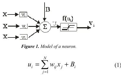
Figure 1. Model of a neuron.
∑
=+
=
Nj
i j ij
i
w
x
B
u
1(1)
In the above model of a neuron (Figure 1) there is a summation element with input signals x x1, 2,...,xN , constituting an input vector
[
x x … xN]
T2 1
=
x . The
components of vector x are multiplied by the weights matched W Wi1, i2,...,WiN. Bi is the bias associated with the node. Out of the summation comes signal ui. During tests, as an activation function, a sigmoid function is accepted, constituting the approximation of a step function. Gradient algorithms are used in the training process, as they are considered the most effective for learning purposes [36].
In preparing data sets to train neural networks, we considered the type of signals used at the input and output of the networks, constituting an input and output vector and determined by the size of the data set for training. In the research under consideration, for the majority of the neural networks the input signal was formed by the external air temperature, while the output signal was its corresponding heat power. In the case of classification: at the input of the network the elements of the object were described, whereas at the output, the result of the classification was stated. In the case of the identification of dynamic objects, at the input of the network the value of an input signal (of the object) was given at the time tn - u(tn ) and at directly preceding times u(tn-1), u(tn-2), ..., while at the output, the value of an output signal (of the object) at a given time was y(tn). In the case of predicting values of time series at the input of the network, signals at the time tn-s(tn) and at preceding times s(tn-1), s(tn-2), ..., s(tn-m), s(tn-m-1), s(tn-m-2) ..., where m stands for a certain period of time (e.g. 24 hours) at the output foreseen signal values s(tn+1), s(tn+2), ... etc. During research one can continuously make adjustments to input and output signals.
When choosing the size of the set, we considered on the one hand the network’s training speed and, on the other, the precision of training. In general, data for training will consist
of many subgroups, each focusing around the determined pattern. Statistical variability must be represented appropriately within each class.
The optimization of the objective function method is used in the network learning procedure. ‘Supervised learning’ – with a teacher – is the most effective method of teaching one-directional sigmoid networks [37]. For the training pair (x, d), the definition of the objective function takes the form of the mean square error:
E
y
d
i M
i i
=
−
=
∑
1
2
12
(
)
(2)where yi=f(ui), f is a sigmoid function. For many training pairs (x(j), d(j)) for j = 1,2, ..., p the definition of the objective function assumes the form:
E
y j
d j
i p
i M
i i
=
−
= =
∑ ∑
1
2
1 12
( ( )
( ))
(3)During this research the method used was based on the choice of direction conforming to the direction of a negative gradient: the algorithm of the steepest descent.
In the second part of the research, the RBT-type of networks was used (Radial Base Functions). In these types of networks a latent neuron plays the function, radially changing around the selected center c. The role of the latent neuron is the radial mirroring of the space around one point or many points. Radial-type networks are complementary to sigmoid networks [37]. A sigmoid neuron constitutes a kind of hyper-plane dividing the multi-dimensional space into two parts for which the following condition is satisfied:
0
>
∑
jj ij
x
W
or∑
j<
0
j ij
x
W
(4)A radial neuron constitutes a kind of hyper-sphere in the middle of which there is the central point.
The use of radial neurons in modelling means that for the case of radial symmetry of the data set, the quantity of data required for classification purposes is reduced considerably. In the case of an excessive quantity of data for training, the system becomes re-dimensioned with too great a number of degrees of freedom, which in effect leads to lower generalizing abilities for the network. As a result, it is necessary to introduce additional ties to limit the degrees of freedom for given parameters. Methods of regularization are used for this purpose. Green’s functions are used most frequently, of which Gauss’s function is the best. The algorithms defined serve as the basis for selecting the quantity of base functions (e.g. Gram-Schmidt ortogonalization), though in this research an empirical selection was made of the quantity of neurons in the hidden layer.
chosen level, this being mainly related to weather conditions. The analysis of the phenomena occurring in one building under consideration and the synthesis of this building’s model will be carried out on the basis of a time series of physical quantities connected with the process of heating the buildings. In effect, the model built (or rather, seeing as neural networks are used as a tool, taught) serves to forecast heat power demand in the form of a time series (power values at given times).
The preparation of input data for the simulation research of the model of identification of the building complex and prediction of heat consumption by these buildings was made possible by the pre-existing computerized system for automatically regulating and monitoring WUT’s main campus. The system was launched in November 1995 and covers the heating system as well as 16 heat substations on WUT’s main campus and a few substations off campus. Each heat substation in the building is equipped with a system to automatically regulate the temperature, feeding the central heating installation depending on external temperature and the system that measures heat consumption. Identification of the building complex was performed using data obtained from the main heat gauge. Data such as temperature, pressure, flows and heat power were read at a frequency of 1-10 minutes and then averaged and committed to memory every hour. These hourly quantities were used to teach and test an artificial neural network. The data gathering took place from 1995 to 2009.
In order to teach the network the dynamics of a system such as the building complex, in which external air temperature constitutes an input signal and heat power demand is an output signal, the following approach was used.
It was assumed: at the output of the network one signal – heat power taken md,h (power was taken on day d at hour h), at the input of the network the values of power taken on the same day one hour, two and three hours earlier (md,h-1, md,h-2, md,h-3), power taken on the previous day, respectively, md-1,h, md-1,h-1, md-1,h-2 , md-1,h-3, power taken two days earlier at appropriate times md-2,h, md-2,h-1, md-2,h-2 , md-2,h-3 and the temperature on the following days and times: td,h, td,h-1, td,h-2, td,h-3, td-1,h, td-1,h-1, td-1,h-2, td-1,h-3, td-2,h, td-2,h-1, td-2,h-2, td-2,h-3.
In the research it was assumed, on the basis of general premises, that a neural network with one hidden layer was in operation. A series of experiments was carried out, teaching and testing networks with a differing number of neurons in the hidden layer. It was established that the best effects were achieved with 25 neurons in the hidden layer of the network. The configuration of the network for research was as follows: 23 neurons in the input layer, 25 neurons in the hidden layer and one neuron in the output layer.
Only networks with back-propagation of error and one hidden layer were used in the research. The number of inputs, neurons in the hidden layer and the number of the network’s outputs, for each of the variants considered, are the outcome of the manner of presenting the data at the input and output
of the network. The tests were performed for 2 different cases:
4.1. Case 1
Four different neural networks were taught and tested. Following the results of research conducted earlier that tested heat power demand prediction for a building complex, new research was carried out using for training purposes an extended database covering 5 heating seasons. For this purpose, a model of a neural network with back-propagation of error with one hidden layer was used. The number of inputs, the number of neurons in the hidden layer and the number of outputs of the network for each of the variants considered result from the means of the presentation of the data at the input and output of the network. The input vector covered 14 types of data and in the hidden layer there were 18 neurons. In the research under consideration, appearing at the input are the following data: external air temperature and heat power taken at times (d – stands for day, h – stands for hour): d,h , d,h-1 , d,h-2 , d-1,h+1 , d-1,h , 1 , d-1,h-2 , d-d-1,h-2,h+1 , d-d-1,h-2,h , d-d-1,h-2,h-1 , d-d-1,h-2,h-d-1,h-2.
At the output of the particular networks, the value of heat power was expected at one hour (d,h+1), two hours (d,h+2) and three hours (d,h+3) in advance. The results of the tests run on the networks taught are shown in Figures 2-4.
Figure 2. Predicted heat power demand 1 hour ahead of time.
Figure 4. Predicted heat power demand 3 hours ahead of time.
The coefficient of variation (CV) is often used as an accuracy measure. The CV is a common metric used for neural networks [24]. Another metric can be correlation coefficient R2 or cross linear Pearson correlation coefficient between observed and predicted date. CV and R2 were estimated for case 1: CV (4.6 %, 6.6 % and 7.3 %) and R2 (0.88, 0.84, 0.82). The results are good, indicating that the neural network parameters were well-selected.
The accuracy and quality of the forecast can be estimated using MSE (mean square error), RMS (root mean error),
Table 1. Forecast errors 1, 2 and 3 hours ahead of time.
MAPE error
Mean error
Max. error
Net-1-hour-advance forecasting 2.9% 0.6% 12.1%
Net-2-hour-advance forecasting 4.1% 1.5% 21.9%
Net-3-hour-advance forecasting 4.7% 4.1% 16.5%
MRE (mean relative error) and others. It is common practice to resort to the Mean Absolute Percentage Error (MAPE) summary measure. It is defined as follows:
∑
=⋅ − = n
i i
i i
y d y
n MAPE
1
% 100 1
(5)
where d is the predicted value, y is the actual value of heat power, n determines the scope for which one estimates forecast error. The following were calculated for all research tests: the mean difference between the actual and predicted value, taking into consideration the deviation mark for the entire measured period and the maximum forecast error estimated for one hour.The MAPE errors, depending on the forecast’s time advance, are in the range 2.9 to 4.7%. Table 1 shows the calculated errors for forecasts of heat power demand 1, 2, and 3 hours in advance.
The longer the forecast period, the lower the accuracy of the forecast. For one-hour- and two-hour-advance forecasts, the mean relative error of 0.6% and 1.5% proves that the neural network is well adjusted to the characteristics of the object under investigation. That is indicative of the fact that heat power demand averaged for the entire measured period is implemented with high accuracy.
4.2. Case 2
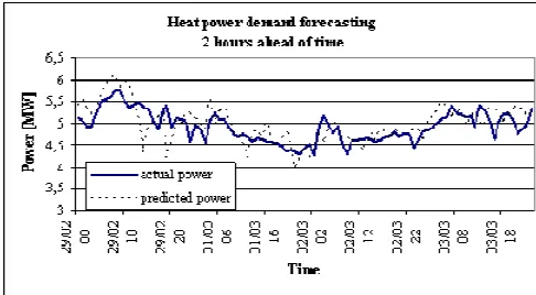
In case 2, for the same input data, neural network models were compared. The comparison concerned the heat consumption model two days earlier and one day earlier with the model analyzing heat consumption only the day before. The aim was to discover whether information about heat consumption in the more distant past significantly influences the heat consumption forecast. Using input data, the research tested many different heat demand forecast variants for WUT’s main campus buildings. The calculated heat consumption values were compared to actual values. Figure 5 shows the result of a one-hour-advance forecast of heat consumption. The data for training and testing included changes in temperature and heat power on the previous day.
Figure 5. Heat power predicted 1 hour ahead of time for a neural network (d-1).
The results presented in Figure 5 can be compared with the results from Figure 6, which were obtained for the same temperature and heat power values though including changes going back one and two days.
Figure 6. Heat power predicted 1 hour ahead of time neural network (d-1, d-2).
Coefficient CV and coefficient R2 were also calculated for case 2. The results were good: CV (2.6 % , 5.3 %) and R2 (0.97 , 0.90).
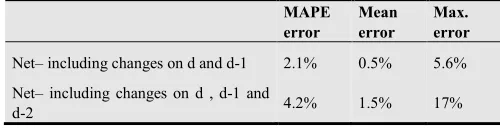
Table 2. Forecast errors for a network including changes 1 day earlier and 1 and 2 days earlier.
MAPE error
Mean error
Max. error
Net– including changes on d and d-1 2.1% 0.5% 5.6%
Net– including changes on d , d-1 and
d-2 4.2% 1.5% 17%
The error for the forecast based on the reference going back one day was 2.1%, and for the forecast going back one and two days it was twice as big, at 4.2%.
Heat demand forecasting is also possible in extreme weather conditions. That entails modelling temperature changes so as to determine heat consumption in these conditions. This may constitute the basis for an update of the power order placed with the district heating company. The condition necessary for using this method is a very large data set for learning, a long training period and a good correlation between obtaining results and the parameters of the training method. Good results prove that the tests the neural network went through were successful. The neural network very accurately reflects the heating characteristics of the buildings on WUT’s main campus.
5. Summary
This research has shown that the forecasting methods employed are a useful tool for steering heat networks and heat sources. The possibility of estimating heat demand a few hours in advance enables optimal determination of the quantity of heat energy to be produced. Adjusting heat production to current demand may boost production system efficiency by as much as a few percent. The use of a model based on artificial neural networks also produced good forecasting results. The choice of the two kinds of networks, namely the back-propagation type and the RBF type (Radial Base Functions), proved appropriate in light of the results obtained from the experiments. The accuracy of the results obtained falls in the range of 3-5%, depending on the kind of network, its architecture, the size and type of input data and the forecast period. For the purposes of steering the heat source, this level of accuracy is sufficient. To satisfy the necessary condition for forecasting heat consumption with the use of an artificial neural network one needs to possess a database of the main heating parameters of a district heating system covering a few years of operation. Research into forecasting the load of a district heating system may be performed for as long as new tools improving prediction quality appear. Neural networks undoubtedly open up new vistas for the discipline and merit use in real life situations.
Symbols
Bi biases,
di i –forecast value, E mean square error [%], M number of training patterns,
md,h heat power taken on day d, at hour h, p number of output neurons,
td,h external temperature on day d, at hour h, ti computational internal temperature [oC], ui output signal,
Wij weight for input signal,
xi empirical value of random variable, yi empirical value of random variable,
References
[1] Report of the President of the Energy Regulatory Office – Heat in Numbers
http://www.ure.gov.pl/portal/pl/pdb/509/Energetyka_cieplna_ w_liczbach.html (in Polish).
[2] Ostergaard P.A., Lund H., A renewable energy system in Frederikshavn using low-temperature geothermal energy for district heating. Applied Energy 88 (2011) 479-487.
[3] Danestig M., Gebremehdin A., Karlsson B., Stockholm CHP potential-An opportunity for CO2 reductions? Energy Policy 35 (2007) 4650-4660.
[4] Directive 2010/75EU of the European Parliament and of the Council of 24 November 2010 on industrial emissions (integrated pollution and control) (Recast).
[5] Directive 2009/29EC of the European Parliament and of the Council of 23 April 2009 amending Directive 2003/87/EC so as to improve and extend the greenhouse gas emission allowance trading scheme of the Community.
[6] Directive 2002/91/EC of the European Parliament and of the Council of 16 December 2002 on the energy performance of buildings.
[7] Directive 2004/8/EC of the European Parliament and of the Council of 11 February 2004 on the promotion of cogeneration based on a useful heat demand in the internal energy market and amending Directive 92/42/EEC.
[8] Directive 2006/32EC of the European Parliament and of the Council of 5 April 2006 on energy end-use efficiency and energy services and repealing Council Directive 93/76/EEC.
[9] Energy Policy for Poland 2030 from 10 of November 2009 (Ministry of Economy – in Polish).
[10] Stevanovic V.D. et al, Prediction of thermal transients in district heating systems, Energy Conversion and Management 50 (2009) 2167-2173.
[11] Larsen H.V. et al, A comparison of aggregated models for simulation and operational optimization of district heating networks, Energy Conversion and Management 45 (2004) 1119-1139.
[12] Lund H., Andersen A.N., Optimal designs of small CHP plants in a market with fluctuating electricity prices, Energy Conversion and Management 46 (2005) 893-904.
[14] Streckiene G. et al, Feasibility of CHP-plants with thermal stores in the German spot market, Applied Energy 86 (2009) 2308-2316.
[15] Energy market http://www.poee.gpw.pl
[16] Ekonomu L., Greek long-term energy consumption prediction using artificial neural networks, Energy 2010; v.35 512-517.
[17] Kreider J.H. et al Operational data as the Basis for Neural Network Prediction of Hourly Electrical Demand. ASHRAE Transactions (102). 1996.
[18] Klajic K. at al, Use of neural networks for modeling and predicting boilers operating performance, Energy 2012; v.45 304-311.
[19] Cay J. at al, Prediction of engine performance and exhaust emissions for gasoline and methanol using artificial neural network, Energy 2013 v.xxx 1-10.
[20] Rohrig K. et al, “New concepts to integrate German offshore wind potential into electrical energy supply” Publication of Institut für Solare Energieversorgungstechnik (ISET). Kassel University 2005.
[21] Kawashima M. at al, “Hourly thermal load prediction for next 24 hours by ARIMA, EWMA, LR and an artificial neural network. ASHRAE Transaction 101 (1), 1995
[22] Neto A.H., Fiorelli F.A, Comparison between detailed model simulation and artificial neural network for forecasting building energy consumption, Energy and Buildings 40 (2008) 2169-2176.
[23] Li K., Su H., Forecasting building energy consumption with hybrid genetic algorithm-hierarchical adaptive network-based fuzzy inference system, Energy and Buildings 42 (2010). 2070-2076.
[24] Kreider F.J,. Wang X.A, “Artificial neural network demonstration for automated generation of energy use predictors for commercial building”. ASHRAE Transaction 97 (1), 1991
[25] Kreider F.J., Haberl J.S., “Predicting hourly building energy use: The great energy predication shoot out – overview and discussion of results”. ASHRAE Transaction 100 (2), 1994
[26] Feuston B.P., Thurtell J.H. “Generalized Nonlinear regression with Ensemble of Neural Nets: The great energy predictor shootout”. ASHRAE Transactions (100). 1994.
[27] Stevenson W.J. “Using Artificial Neural Nets to Predict Building Energy Parameters”. ASHRAE Transactions (100). 1994.
[28] American Society of Heating, Refrigeration and Air-Conditioning engineers, Inc. “The Use of Artificial Intelligence in Building Systems”. A Collection of Papers from ASHRAE Transactions and ASHRAE Journal. Atlanta 1995r.
[29] Haberl J.S., Thamilseran S. “The great energy predication shoot out II. Measuring retrofit savings - overview and discussion of results”. ASHRAE Transaction 102 (2), 1996
[30] Fast M., Palme T. “Application of artificial neural networks to the condition monitoring and diagnosis of a combined heat and power plant”. Energy 35 (2010) 1114-1120.
[31] Ahmed O. et al, “Feedforward-Feedback Controller Using General Regression Neural Network (GRNN) for Laboratory HVAC System”. ASHRAE Transactions. 1998.
[32] Curtis P.S. et al, “Adaptive control of HVAC Processes using Predictive neural networks”. ASHRAE Transactions (99). 1993.
[33] Kalogirou S., Bojic M. “Artificial neural networks for the prediction of the energy consumption of a passive solar building”. Pergamon. Energy no 25 /2000.
[34] Privara S. at al, “Model predictive control of a building heating system: the first experience”. Energy and Buildings 43 (2011) 564-572.
[35] Chmielnicki W. “Application of neural networks for control of district heating”. Archives of Civil Engineering. PWN. Volume 56, issue 3. Warsaw 2010.
[36] Osowski S. “Neural networks – algorithmic approach” WNT, Warsaw 1996. (in Polish).