613 | P a g e
ROADWAY CAPACITY ESTIMATION BY
MICROSIMULATION MODELLING
Anirudh Rao Katapadi
1, Chethan Kumar N T
2,Mithun
31
Project Consultant, &Civil Engineer, PROJECTILE, Mangaluru, Karnataka, (India)
2Assistant Professor, Civil Engineering Department, SCEM, Mangaluru, Karnataka, (India)
3Assistant Professor, Civil Engineering Department, PACE, Mangaluru,Karnataka, (India)
ABSTRACT
Road network planning and analysis need a lot of data, right from road alignment to the traffic forecasting. Extensive traffic studies are required to carry out accurate data collections which are costly. The traffic scenario in the developing countries like India is heterogeneous traffic which adds to the difficulty in data collection and therefore modelling holds a lot of relevance in understanding the various parameters of traffic flow. Traffic simulation offers a very effective alternate to the conventional practices of elaborate field data collection.
The present study is aimed at understanding the traffic scenario on straight road sections on urban roads. Traffic flow parameters are obtained from three sections viz., Kulur-Ferry Road, M.G. Road & Airport Road. PCU values are computed for the prevailing heterogeneous traffic conditions for all the sections. Correlation between traffic parameters of flow, speed and density are carried out. VISSIM 8.0 microscopic simulation software is used to develop the traffic model and simulation data is compared with field data.
Key Words: Micro simulation, PCU and model
I. INTRODUCTION
1.1General
Transportation is an important aspect in today’s world. Economic development of any region has close
dependence with the transportation systems. Transport planning and forecasting, are vital for further
improvement in the transport network and inter-mode. Transport Planning is an integral part of any town and
country planning.
Road-user behaviours are linked to various physiological and vehicular characteristics. There is a continual
problem confronting the transportation stakeholders with the evolving vehicular systems. Technologies in
vehicles are evolving faster than the road networks. Vehicular characteristics like acceleration, power, braking
properties, the vehicular dimensional configuration etc. have a bearing in arriving at a very important index
called the Passenger Car Unit.
It is well established that modern civilization has been engulfed in two primary features of globalization and
industrialisation. There has been unprecedented growth in traffic and often the roads are getting congested
leading to traffic jam. The pattern of urban sprawl is changing. A lot of measures are being contemplated by
614 | P a g e
1.2 Statement of Problem
Transportation network is confronted with many complex problems. Capacity estimation is a dynamic problem.
Vehicle density is increasing every year and is leading to congestion on many roads. Vehicle shapes and
characteristics are changing rapidly. Therefore study of road traffic essentials like planning, designing of
roadway, operations of roadway facilities along with control and regulation become necessary. On field
observations and data collection and analysis is tedious and time consuming. Broad spectrum collection of data
collection is therefore very difficult. Modelling of traffic flow is a time-tested alternate.
Generally, in developing and under developing nations the nature of traffic is heterogeneous. There is no
separation of traffic and all vehicles share the same space. Direct adoption of traffic parameters of different
countries is not a viable solution. Modifications to PCU would enable more realistic outcome. Unrestricted
movements of vehicles make the lane concept, flow values parameters taken from standard lane width invalid.
1.3 Main Objectives and Scope of Present Study
Direct adoption of traffic parameters from homogeneous conditions to suit the heterogeneous conditions is not
the best solution. Systematic approach to determine PCU, flow, density, speed and capacity are absolutely
necessary. The objectives of the study are enlisted below.
1. To determine the roadway capacity of straight section.
2. To obtain speed-flow-density parameters.
3. To compare both macroscopic and microscopic simulation method.
4. To understand traffic patterns on the study sections.
1.4 Scope of the Study
This study is aimed at traffic data collection on three important urban arterial roads. Kulur-Ferry road is the first
study section and is one of the important roads of the city. This road is a divided carriageway with pedestrian
footpaths on either side. Second study section is M.G. road which extends from PVS intersection to Lady hill
rotary intersection. Airport Road is the third road section where the traffic parameters have been captured.
Broadly the road geometrics are the same and the roads are at grade. The scope of the study includes collection
of traffic parameters of speed, volume, vehicle characteristics, and roadway parameters.
II.STUDY METHODOLOGY
2.1 Experimental procedure
Data collection is a very important step. It should be very efficient to proivde all the data required for analysing
the traffic flow. There are several techniques available for traffic study. The choice of method depends on the
importance and the extensiveness of the data required. The duration of the count depends on the purpose and the
requirements of the traffic engineer. The following are the methods of data collection
1. Mechanical method
615 | P a g e
3. Combination of mechanical and manual method
4. Automatic devices
5. Moving observer method
6. Photographic method
7. Video recording method
2.2 Mechanical Method
Mechanical methods are broadly classified into intrusive method and non-intrusive method. These methods are
generally expensive in comparison with other methods. The intrusive methods comprises of a data recorder and
a sensor. The non-intrusive methods are passive and active infra-red method, passive magnetic method, micro
wave radar method, ultrasonic and passive acoustic method.
2.3 Manual Method
Manual method is perhaps the oldest methods of traffic counting. The number of observers needed to count the
vehicles depend on the number of lanes from which information is to be collected.
2.4 Combination of Mechanical and Manual Method
A primitive example of this method is multiple pen recorders. A display chart moves continuously at speed of
clock. Pressing of the switch actuates the pen recorder. Simultaneous operations of classification and count are
performed.
2.5 Automatic Devices
These devices facilitate large volume data extraction with high degree of accuracy. Generally, traffic counts are
taken on hourly basis on a 24-hour time schedule. This method is suited to identify the peak hour traffic and jam
density.
2.6 Photographic Method
Techniques such as stereo-continuous strip photography and time lapse photography have been found extremely
useful for traffic engineers. Aerial photographs have been captured for carrying traffic analysis. This technique
allows for greater accuracy of data collection.
2.7 Video Recording Method
This method offers great varsatility. Video on a 24-hour tie interval can be captured and frame by frame analysis
is possible with high end video recorders.
III.RESULTS AND DISCUSSIONS:
3.1 Development of Base Network
Background maps are used to setup the VISSIM network to scale. Hence it is important to place and scale
background images correctly. Links and connectors are very important in development of road network and is
616 | P a g e
turning movements assignments are to be completed. Traffic volumes, classification and vehicle classesdepending on the extracted field data are entered.
3.2 Traffic Categories
By default VISSIM doesn’t have most of the Indian vehicle categories; therefore it is necessary to create an
Indian vehicle categories required for the present study. Vehicle categories like 2 wheelers, motorized 3
wheelers, Car, LCV, Buses and trucks are created in VISSIM for the further study
.
3.3 Traffic Flow and Composition
Traffic volume has to be given from the collected traffic volume count form the field at different time interval.
Vehicular composition extracted from the classified traffic volume count has to be given as input. Desired speed
distribution is also one of the inputs at this stage. VISSIM would generate random traffic volume and vehicle
composition from the given data. Figure 3.3 shows the vehicle compositions and relative flow input. Example
showing traffic volume input and selection of vehicle composition type for particular study section.
Plate 3.1 Representation of Vehicle Input
3.4 Desired Speed Distribution
Based on the observed data, minimum speed, maximum speed and their distribution of each vehicle type has to
be given as input in VISSIM. In the present study speed distribution has been plotted for all the vehicle
categories for both horizontal curved section and straight section separately. Figure 3.2 shows the desired speed
distribution graph for car
.
617 | P a g e
3.5 Driving Behavior Parameter
As discussed earlier in this chapter Wiede mann 74 car following model’s three driving beha viour
parameters are average stand still distances, additive part of safety distance, multiplicative part of safety
distance. In the present study by changing the value of these parameters traffic models are calibrated for
all the section. Table 3.1 lists the default driving behaviour parameters of VISSIM
Description of the Parameter Default Value
Average standstill distance 2m
Additive part of safety distance 2m
Multiplicative part of safety distance 3m
Table 3.1 Default Driving Behaviour Parameter
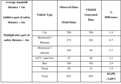
3.6 Calibration and Validation of Simulation Model
After input of all the parameters are completed, it is necessary to calibrate and validate the simulation model. By
modifying the driver behaviour parameters using iterative method, VISSIM simulation model is calibrated.
Simulation model is then validated by comparing the observed classified volume count and obtained traffic
volume count from the VISSIM. Table 3.2 lists the traffic flow validation for site 1.
Average standstill
distance = 1m
Vehicle Type
Observed Data
VISSIM
Generated
Data
%
Difference Additive part of safety
distance = 1m (Field Data)
Multiplicative part of
safety distance = 2m
Car 290 294 1.4
Motorized 2
Wheeler 279 281 0.7
Motorized 3
wheeler 105 99 5.7
LCV / mini bus 47 46 2.1
Bus 104 101 2.9
Truck 30 31 3.3
Total 855 852 MAPE
=2.68%
618 | P a g e
Table shows the MAPE value is 2.68% that means obtained values for particular driver behavior parameters areaccurate and within acceptable limits. Similarly, MAPE value for site 2 is 3.63% and for Airport Road is 2.90%.
Roadway Capacity Estimation by Micro Simulation Approach
Once the classified traffic volume is obtained from the VISSIM simulation, by modified density method
volumes which are in vehicle per hour are converted into PCU per hour. PCUs obtained from the modified
density method are multiplied by number of that vehicle type and then these values are added to obtain the total
volume in PCUs in that
five minutes interval. To obtain the flow values in PCU/hour, the volume
obtained for 5 minutes is
multiplied with 12 (number of 5 minutes in an hour). Speed – flow – density curvesare drawn for obtained values from VISSIM and optimum capacity has been calculated.
Optimum capacity obtained from modified density method, speed area method and microscopic simulation
methods for all the test sections are listed in Table 3.3
Road Section
Optimum Flow PCU/hr
Speed Area Method Microscopic Simulation Method
Site 1 1550 1470
Site 2 1865 1835
Site 3 1900 1865
Table3.2. Roadway Capacity
IV. CONCLUSSION AND SCOPE FOR FUTURE STUDIES
The findings from the study are presented below.
1. In the present study, the optimum roadway capacity observed on three straight sections was calculated using
the macroscopic and microscopic approaches.
2. It has been seen from the macroscopic analysis; it is evident PCU values of vehicles are dependent on the
traffic composition.
3. Traffic volumes obtained from the macroscopic analysis are showing good correlation with microscopic
analysis.
4. Traffic volumes from microscopic analysis are showing same trend as macroscopic approach
5. In the present study PCU values are calculated from speed area method. Hence, it is proposed to attempt to
use Area Occupancy method and Modified Density method.
6. Impact of lane changing behaviour on traffic flow can be analysed.
7. Microscopic simulation study can be performed by using other traffic simulation software and methods.
619 | P a g e
Highway Capacity Manual 2000[1] IRC: 106-1990 - Guidelines for capacity of urban roads in plain areas.
[2] Satish Chandra and Upendra Kumar,(2002) “Effect of Lane Width on Capacity under Mixed Traffic
Conditions In India” Journal of Transportation Engineering, Vol. 129,no 2
[3] V. Thamizh Arasan and Shriniwas S. Arkatkar, (2010) "Micro-simulation Study of Effect of Volume and
Road Width on PCU of Vehicles under Heterogeneous Traffic". 1110 / Journal of Transportation Engineering © ASCE / December 2010.
[4] S. VELMURUGAN et. al. (2010) "Critical Evaluation of Roadway Capacity of Multi-Lane High Speed
Corridors Under Heterogeneous Traffic Conditions Through Traditional and Microscopic Simulation
Models". Journal of the Indian Roads Congress, October-December
[5] Hashim Ibrahim Hassan, Abdel-Wahed Talaat Ali, (2012) "Effect of Highway Geometric
Characteristics on Capacity Loss". Journal of Transportation Systems Engineering and Information Technology Volume 12, issue 5.
[6] Prema Somanathan Praveen, Venkatachalam Thamizh Arasan, (2013) "Influence Of Traffic Mix on PCU
Value of Vehicles under Heterogeneous Traffic Conditions". International Journal for Traffic and Transport Engineering.
[7] Joonhyo Kim, Lily Elefteriadou (2009), “Estimation of Capacity of Two-Lane Two-Way Highways Using
Simulation Model”. Journal of Transportation Engineering, Vol. 136, No. 1, January 1. ©ASCE
[8] Shriniwas S. Arkatkar, V. Thamizh Arasan (2012), “Micro-simulation Study of Vehicular Interactions on