www.nat-hazards-earth-syst-sci.net/14/3143/2014/ doi:10.5194/nhess-14-3143-2014
© Author(s) 2014. CC Attribution 3.0 License.
Time–frequency analysis of the sea state
with the Andrea freak wave
Z. Cherneva and C. Guedes Soares
Centre for Marine Technology and Engineering (CENTEC), Instituto Superior Técnico, Universidade de Lisboa, Av. Rovisco Pais, 1049-001 Lisbon, Portugal
Correspondence to: C. Guedes Soares ([email protected])
Received: 21 August 2013 – Published in Nat. Hazards Earth Syst. Sci. Discuss.: 14 February 2014 Revised: 17 September 2014 – Accepted: 10 October 2014 – Published: 1 December 2014
Abstract. The nonlinear and nonstationary properties of a special field wave record are analysed with the Wigner spec-trum with the Choi–Williams kernel. The wave time series, which was recorded at the Ekofisk complex in the central North Sea at 00:40 UTC (universal time coordinated) on 9 November 2007, contains an abnormally high wave known as the “Andrea” wave. The ability of the Wigner spectrum to reveal the wave energy distribution in frequency and time is demonstrated. The results are compared with previous in-vestigations for different sea states and also the state with Draupner’s abnormal “New Year” wave.
1 Introduction
Several events in which ships have been damaged by giant waves have been reported in the literature during the last 20 years (e.g. Kjeldsen, 1997; Faulkner and Buckley, 1997). The interest in this type of waves have lead to the analysis of data from real sea states, i.e. looking for occurrences of abnor-mally high waves, which have been reported in an increasing number of works. Instrumental records have identified this type of wave in the North Sea (Skourup et al., 1996; Haver and Andersen, 2000; Wolfram et al., 2000; Guedes Soares et al., 2003; Magnusson and Donelan, 2013), the Sea of Japan (Yasuda and Mori, 1997; Mori et al., 2002), the Gulf of Mex-ico (Guedes Soares et al., 2004) and even in the Baltic Sea (Didenkulova, 2011). A more comprehensive review of reg-istered huge waves is made in Kharif et al. (2009).
Waves of anomalously large size, called abnormal, freak, or rogue waves, are very steep in the last stage of their evo-lution and propagate as a wall of water. A typical abnormal
wave is a single event with a characteristic lifetime of just a few seconds. Before breaking, it has a crest 3–4 times higher than the crests of neighbouring waves and appears almost in-stantly, as it has been identified in wave records. There is no doubt that such waves are essentially of nonlinear character and can be generated by different mechanisms (Kharif et al., 2009).
Understanding the nature of abnormal waves can be achieved by a detailed analysis of the time records of free surface elevation using different methods to determine their time–frequency energy distributions.
The standard Fourier analysis is a powerful tool for the in-vestigation of waves because it provides the opportunity to decompose the series into individual frequency components and to specify their relative intensity. However, the usual fre-quency spectrum does not give any information when these frequencies bring a great amount of energy. The assumption is that it happens in the same manner during all periods of measurement.
Visual observation of the sea surface shows that the wind waves of various heights move in reiterated groups of differ-ent length and number of waves. This means that for short time intervals nearly equal to the group duration there exists significant change of the wave energy per unit square surface. Therefore, the wind wave for short intervals of time is not a stationary process as is usually supposed.
explanation of the physical and mathematical ideas for un-derstanding what is changeable in the time spectrum. The main idea is to find a joint function of frequency and time that describes the energy distribution of the process. In the ideal case such distribution will be used and transformed in a same manner as any joint distribution. Nevertheless, the joint functions in frequency and time of the wave en-ergy are not distributions in a probabilistic sense because the time–frequency spectra provide a distribution of the en-ergy while probabilistic joint distribution of two variables de-scribes their joint probability. However, for historical reasons the time–frequency spectra of the signals are often also called “distributions”.
The previously mentioned authors lead their works by a partial mathematical similarity with some problems in quan-tum mechanics and signal processing. It is necessary to high-light clearly that the analogy between quantum mechanics and the theory of signals is formal and that the physical inter-pretation in these two branches of knowledge is completely different (Cohen, 1995).
First, Gabor (1946) developed the mathematical basis of the time–frequency method and introduced a very impor-tant concept for analytical signal that is later applied in ra-diophysics and the theory of signals. Furthermore, (Turner, 1954; Levin, 1967) it is shown that using procedures simi-lar to those in the work of Page (1952) it is possible to find many other time–frequency distributions. Rihaczek (1968) deduced a new distribution examining problems of physics connected with signals spreading. A lot of ideas about the convolution and filtering of the nonstationary stochastic pro-cesses are introduced in the detailed work of Mark (1970) and are now applied in the everyday practice of many scien-tific fields.
The last 2 decades of the 20th century mark a great progress of investigations dedicated to the time–frequency structure of the signals. This revival of the scientific interest (Claasen and Meklenbruker, 1980a, b, c; Janse and Kaizer, 1983) is accompanied with the development of unique ideas of the spectral distributions and demonstrates their practi-cal application. Moreover, it begins to clarify the similar-ity and difference between the quantum mechanics and the theory of the real signals. In the works of Boashash and Whitehouse (1986) and Boles and Boashash (1988), the ideas developed by Claasen and Meeklenbräuker (1980a, b, c) are implemented, possibly for the first time, to deal with the real problems of geophysics.
In the course of time a new manner of thinking arose for the interpretation and use of the time–frequency energy dis-tributions. Different points of view and different scientific interests extend the understanding of what the nonstation-ary processes are and diversify the techniques of their inves-tigation. A good review of the applied and scientific prob-lems connected with time–frequency analysis can be found in Cohen (1995), Hlawatsch and Boudreaux-Bartels (1992),
Boashash (1991), Meecklenbräuker (1985), Hlawatsch and Flandrin (1992) and Huang et al. (1998).
Some of time–frequency energy distributions are already used to study the nature of the ocean wind waves such as wavelet distribution (Liu, 1994, 2000 a, b; Massel, 2001), spectrogram distribution (Guedes Soares and Cherneva, 2005; Cherneva and Guedes Soares, 2005), the empirical mode decomposition (Huang et al., 1998; Schurlman, 2001; Veltcheva and Guedes Soares, 2007, 2011) and Wigner spec-tra (Cherneva and Guedes Soares, 2008, 2011, 2012).
The present study analyses sea state wave data from sin-gle point measurements, in order to characterize the nonsta-tionary and nonlinear properties of the large waves regis-tered in the North Sea at the Andrea platform. It is a follow-up to a series of studies performed (Guedes Soares et al., 2003, 2004; Guedes Soares and Cherneva, 2005; Cherneva and Guedes Soares, 2008, 2011, 2012; Veltcheva and Guedes Soares, 2007, 2011). In what follows, Sect. 2 provides a theo-retical background to presenting wind waves as an analytical process, introduces a definition of a Wigner spectrum and briefly describes the Benjamin–Feir instability. Results and discussions are the subject of Sect. 3. Conclusions are made in Sect. 4.
2 Theoretical background
2.1 Wind waves as an analytical process
It was already mentioned that the concept for the analytical signal belongs to Gabor (1946). After the pioneering work of Longuet-Higgins (1952), mathematical and physical meth-ods from radiophysics, theory of noise and signal processing are widely introduced in the investigation of wind waves (e.g. Bitner, 1980; Bitner-Gregersen and Gran, 1983; Tayfun and Lo, 1989).
Ifη(t )is the surface elevation andη(t )˙ is its Hilbert trans-form, the complex processx(t )=η(t )+jη(t )˙ is an analyti-cal process, corresponding toη(t ). The processx(t )can be presented also asx(t )= |A(t )|exp[j ψ (t )], where the enve-lope|A(t )|and the phaseψ (t )are defined as
|A(t )| =hη˙2(t )+2(t )i1/2, (1)
ψ (t )=arctg[ ˙η(t )/η(t )]. (2)
The phaseψ (t )can also be written as
ψ (t )=ω0t+ϕ(t ), (3)
whereω0is co-called carrier frequency andϕ(t )is the local phase. The time derivative of the phase functionψ (t )defines a local frequency of the time series:
In this sense, the local frequencyω(t )is a rate of change of the phase (Van der Pol, 1946). If it is assumed that at each time instantt there exists only one single frequency compo-nent the local frequency is defined also as an average fre-quency at a particular time. Then the sea state is restricted to a single mean wave characteristic, such as the local fre-quency, which changes in time.
In Eq. (3) the unwrapped phase functionψ (t )consists of a linear partω0tincreasing with time and a deviation partϕ(t ) superimposed onω0t. Therefore, from the slope of the un-wrapped phase functionψ (t )it is possible to find the carrier frequencyω0. It is obvious that the carrier frequencyω0does not coincide with the spectrum peak frequencyωp. Usually ωpis less thanω0for the real sea state spectra and the fact is not connected with downshifting of the spectrum peak fre-quency due to Benjamin–Feir instability. Only when waves have nearly equal phases during a given time interval and the change of the phases in timeθ=dϕ(t )/dt is small, the local frequency is equal to the carrier frequencyω0. If the phase change has negative slope θ=dϕ(t )/dt <0, then the local frequency is lower than the carrier one. A detailed discussion about the local frequency of the signal can be found in the classic work of Cohen (1989).
2.2 Wigner spectrum
For the analytical signal x(t ), Fonolosa and Nikias (1993, 1994) define the Wigner high-order time–frequency spec-trum as
Wkx(t, f1, . . ., fk)=
Z Z Z
uτ1 . . .
Z
τk
8 (, τ1, . . ., τk)
×Rku(τ1, . . ., τk)exp(2πj u)exp(−2πj t ) (5)
×
k
Y
i=1
exp(−j2π fiτi)dτidud.
HereWkx(t, f1, . . . ,fk)is ak-dimensional Fourier transform
of ak-dimensional local moment functionRku(τ1, . . . , τk),
and 8(, τ1, . . . , τk) is a kernel introduced to reduce
the aliasing. The definition (Eq. 5) is preferred because it allows for an opportunity to estimate the higher-order time–frequency spectra of the waves as it was done before for the “New Year wave” (Cherneva and Guedes Soares, 2008).
For k=1, Eq. (5) leads to a definition of the Wigner spectrum. The most applied time–frequency Wigner spec-tra can be obtained using different kernels 8(, τ ). In particular, the Wigner–Ville distribution corre-sponds to 8(, τ )=1 and the Rihaczek distribution to 8(, τ )=exp(j π τ ) (Cohen, 1966). Here the Choi–Williams kernel 8(, τ )=exp(−2τ2/σ ) is used, whereσ=0.05 (Choi and Williams, 1989).
2.3 Benjamin–Feir instability
Ocean waves in their nature are nonlinear and dispersive waves. Experimental studies of Benjamin and Feir (1967) show that regular wave trains in deep water are responsible for a number of instabilities now known as Benjamin–Feir in-stability. The instability is a result of an interaction between three monochromatic wave trains: carrierωc, upperω+ and lowerω−sideband waves. According to a perturbation anal-ysis accomplished by Benjamin and Feir (1967) based on the Euler equations, ifδ ωis a small frequency perturbation, then the carrier wave and the sideband waves have to meet the re-quirements to four wave-resonance conditions for infinitesi-mal waves where
ω±=ωc±δω,
2ωc=ω++ω−, (6)
2kc=k++k−+1k.
In Eq. (6) the frequencies and the wave numbers are con-nected by the linear dispersion relationship in deep water and 1k is a small mismatch. The group of three waves with initial carrier wave amplitude ac is unstable if the inequality 0<δˆ≤
√
2 is satisfied, where δˆ=δ ω/ε ωc and ε=ackc. Then the sideband waves begin to grow in am-plitude at the expense of the main wave. The maximum βx=d(lna)/d(k x) appears when δˆ=1.0 and the initial
phases of the sidebands are ψ±= −π/4. This theory is in good agreement with observations for wave steepnessεin the interval [0.07, 0.17] (Benjamin, 1967).
The evolution of a nonlinear wave train without dissipation manifests the so-called Fermi–Pasta–Ulam phenomenon: pe-riodically increasing and decreasing the modulation causing the wave to return to its initial form (Lake et al., 1977). Fur-thermore, Longuet-Higgins (1978) found that subharmonic instabilities of the Benjamin–Feir type are restricted to waves whose steepnessε=a khas an upper limit. As εincreases beyond 0.346 the wave modes become stable again.
Tulin and Waseda (1999) compared their experimen-tal data with the theoretical predictions of Benjamin and Feir (1967) and Krasitskii (1994). They found that Kra-sitskii’s modification of the Zakharov evolution equation (Zakharov, 1968) correctly predicts the major features of the energy increase in the lower sideband relative to the upper sideband. Additionally, they argued that downshifting to a lower sideband of the spectral peak also appears in the ab-sence of breaking, and showed the significant role of the bal-ance between momentum losses and energy dissipation in the exchange of energy between the sidebands.
Table 1. Parameters characterizing the nonlinearity of the series and of the individual freak waves.
Quantity Hs, m kph ε=askp as/ h Hfreak, m Tfreak, s εfreak kfreakh afreak/ h
Andrea 9.18 1.61 0.106 0.066 21.14 12.0 0.295 1.9543 0.151 Draupner 11.92 1.96 0.081 0.085 25.01 13.1 0.293 1.640 0.179
3 Results and discussion
Here a wave time series measured at 00:40 UTC (universal standard time) on 9 November 2007 is analysed. The series containing a huge wave named the “Andrea” rogue wave was recorded at the Ekofisk complex operated by ConocoPhillips in the central North Sea (56◦300N, 3◦120E), where the water depth is between 70 and 80 m. A detailed description of the weather conditions, measuring installations and some com-parisons between the Draupner’s New Year wave and the An-drea wave can be found in Magnusson and Donelan (2013). Table 1 shows some of the data in that paper with some of the present results.
Table 1 presents the three parameters characterizing the nonlinearity of the series with freak waves measured at the Draupner and the Andrea platforms:kph,ε=askpandas/ h, whereas=Hs/2,his the depth,Hs is the significant wave height and kp is the wave number of the spectrum peak frequency. Similar parameters but for the individual abnor-mal waves, noted with the subscript “freak”, are also cal-culated, where Hfreak is the height of the freak wave and afreak=Hfreak/2;Tfreak is its individual period andkfreak is the wave number corresponding to that period. The steepness of the series is 0.081 for the New Year wave and 0.106 for the Andrea wave. The individual steepness of the rogue waves is εfreak≈0.3, which is less than the upper limit of 0.346 (Longuet-Higgins, 1978). For freak waves the parameters kfreakh≈2, andafreak/ h≈0.2; from this it can be concluded that the registered two abnormal waves are strongly nonlinear (Kurkin and Pelinovsky, 2004; Cherneva and Guedes Soares, 2008).
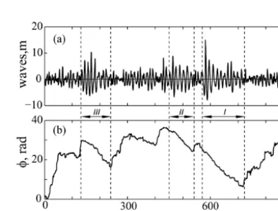
The available Andrea time series has 4600 registered ordi-nates with a 5 Hz sampling frequency that gives 15 min du-rations of the registration presented in Fig. 1a. The existence of foam or possible breaking is taken into account as it is described in Magnusson and Donelan (2013). The series is too short to derive any conclusion about the distribution of the wave heights or crests as done in Cherneva et al. (2009, 2013). Because of that, in this work the study is limited to nonlinear and nonstationary properties of the waves.
There are three high-wave groups which are interesting and investigated here: the first one is a long group in the time interval of 560–720 s containing a huge wave in its begin-ning; the second group exists in the interval of 420–540 s; waves in the third group of the interval of 130–200 s are high, as the waves in the second group, but do not have the typi-cal triangle structure as in the first two groups. In Fig. 1a the
Figure 1. Andrea freak wave. (a) Series measured at 00:40 UTC on
9 November 2007; (b) phaseϕin time.
groups are separated from the rest of the series by vertical dashed lines.
In Fig. 1b one can find the phaseϕdevelopment in time. The phaseϕcan be approximated by straight lines with nega-tive slopes during the investigated group intervals. It is obvi-ous that the local frequencyω(t )of the largest wave groups is smaller than the calculated carrier frequencyω0of the se-ries because dϕ(t )/dt <0. Between the high groups there are time intervals when the amplitudes are very small and a significant positive phase change is registered which is manifested by jumps ofϕ. Such jumps have been observed previously in Guedes Soares and Cherneva (2005) for the waves in deep water near the Portuguese coast. Studying the evolution of nonlinear wave trains, Melvill (1983) first suggests that “crest pearing” (Ramamonjiarisoa and Mollo-Cristensen, 1979; Mollo-Cristensen and Ramamonjiarisoa, 1982) may appear as a result of large positive gradients in phase speed when one crest overtakes the previous.
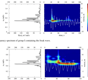
Figure 2. Time–frequency spectrum of group I containing the freak wave.
Figure 3. Time–frequency spectrum of group II between 440 and 520 s.
distribution. Spectrum and time–frequency spectra are calcu-lated with same frequency resolution.
The Wigner spectrum of the group containing the Andrea freak wave is presented in Fig. 2. During the abnormal wave the energy is distributed in a wide frequency interval. There are several peaks that coincide with the corresponding peaks of the usual frequency spectrum. The group has the typical triangle form for the nonlinear waves.
Investigating the nonlinear high waves and the group de-velopment in the tank, the triangle group form has been regis-tered many times (Cherneva and Guedes Soares, 2012). The form is a result of continuous shrinking of the group at differ-ent distances from the wave maker and of changing the place of the highest wave from the middle to the front of the group. For the tank-produced waves, the process is accompanied with frequency downshifting of the energy peak inside the group demonstrated by the time–frequency spectrum. The group is extremely short at the point of focus and has a form similar to the New Year wave group. Moving forward, the focus the group disintegrates and the time–frequency spec-trum shows frequency upshifting of the energy peak. The same character of group development with distance is noted by Kharif et al. (2008) in their investigation of the wind’s influence on the wave groups at different wind velocitiesU (includingU=0) and distances.
It has to be remarked that there is no registered downshift-ing of the energy maximum of the time–frequency spectrum of the group containing the Andrea abnormal wave. In a spec-trogram analysis of real sea states it was also noticed that not all groups demonstrate frequency downshifting of the energy. A similar conclusion was obtained by Su (1982), who inves-tigated the gravity wave group evolution with moderate and high steepness.
It is also necessary to mention that a frequency upshifting like the one for the groups in the tank after the focus is not registered in real sea states.
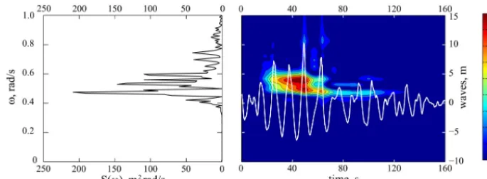
Figure 4. Time–frequency spectrum of group III between 130 and 235 s.
Figure 4 shows the Wigner spectrum of the group that ex-ists in the time interval of 130–235 s (see Fig. 1a). The phase rate for that group is not constant and slowly changes in time. The picture of the peaks registered in the time–frequency spectrum of the group is very interesting. The first three waves have heights of less than 3 m. Their energy peaks are less than 10 % of the highest peak during the group’s lifetime and are invisible. The fourth and the fifth waves have the energy peak of the same frequency. The energy of that peak increases with time. It reaches its maximum value during the highest wave of the group and drastically decreases for the next waves. A second peak of lower fre-quency than the first one during the highest wave appears. It begins to dominate the energy distribution in the lifetime of the next waves. Weak downshifting of that second peak is observed since it reaches the frequencyωp. A similar type of frequency downshifting during the group’s lifetime has al-ready been observed (Guedes Soares and Cherneva, 2005) for a two-wave system sea state without abnormal waves, a broad spectrum and a small angle between the main direc-tions of the system. The peak in the higher frequency of one wave system shifts to the low frequency and unites with the peak of the second wave system. It can be suggested that the complicated time–frequency spectrum picture of group III in Fig. 1b is possibly a result of the interaction of wave compo-nents coming from separate directions. As Magnusson and Donelan (2013) note, “the Andrea wave is observed just past 00 UTC, after a stable period with less wind forcing, but at the start of a new wind increase from a new and slightly dif-ferent direction”.
4 Conclusions
The example of the Andrea series was measured in harsh meteorological conditions and has a higher steep-ness than previously analysed waves by Guedes Soares and Cherneva (2005). The abnormal Andrea wave exists in a large group of 12 waves and differs from the New Year wave which exists in a group similar to the well-known “three sisters”.
Here, the time–frequency analysis is made with a more sophisticated Wigner spectrum but shows a similar charac-ter of energy distribution during the group’s lifetime as that traced out by spectrogram analyses. It is revealed that during the highest wave of the group, the energy spreads in a wide frequency interval with several peaks and confirms the pre-vious results for the abnormal Draupner wave (Cherneva and Guedes Soares, 2008).
The abnormally high Andrea wave is registered in a wave group having a constant local frequency. That local fre-quencyω(t )is less than the calculated carrier frequencyω0 of all series using Eq. (4). In time, the abnormal wave hap-pens at exactly the moment in which the series’ highest peak of energy exists and has frequency equal to the frequencyωp of the usual stationary spectrum.
Not all groups investigated in real sea states demonstrate a frequency downshifting of the energy with time. For exam-ple, the long group that contains the Andrea freak wave has no frequency downshifting of that type registered in the Mar-intek tank. Also, frequency upshifting like that marked after the focus for the in-tank groups is not registered in real sea states investigated by the authors.
The energy distribution in time of the groups that have a changeable local frequencyω(t )is more sophisticated. The waves in such groups are not very steep, but in the time inter-val when the highest waves exist a significant downshifting of the local spectrum peak is observed. It is realized by a jump during the highest wave. It is suggested that more com-plicated downshifting is possibly a consequence of the inter-action of wave components coming from separate directions.
Acknowledgements. The present work had been partly supported by EU contract no. SCP8-GA-2009-234175, EXTREME SEAS – Design for Ship Safety in Extreme Seas.
References
Benjamin, T.: Instability of periodic wave trains in nonlinear disper-sive systems, P. Roy. Soc. Lond. A, 299, 59–76, 1967.
Benjamin, T. and Feir, J.: The Disintegration of Wave Trains on Deep Water, Part I, J. Fluid Mech., 27, 417–430, 1967.
Bitner, E.: Non-linear effects of the statistical model of shallow wa-ter wind waves, Appl. Ocean Res., 2, 63–73, 1980.
Bitner-Gregersen, E. and Gran, S.: Local properties of sea waves defined from a wave record, Appl. Ocean Res., 5, 210–214, 1983. Boashash, B.: Time-Frequency Signal Analysis, in: Advances in Spectrum Estimation, edited by: Haykin, S., Englewood Cliffs, Prentice Hall, NJ, 418–517, 1991.
Boashash, B. and Whitehouse, H.: Seismic applications of the Wigner-Wille distribution, Proc. IEEE Conf. Systems and Cir-cuits, San Jose, USA, 34–37, 1986.
Boles, P. and Boashash, B.: The cross Wigner-Ville distribution – a two-dimensional analysis method for the processing of vibroseis seismic signals, Proc. IEEE ICASSP, 87, 904–907, 1988. Cherneva, Z. and Guedes Soares, C.: Bispectra and time-frequency
spectra of wind waves in the coastal zone, in: Maritime Trans-portation and Exploitation of Ocean and Coastal Resources, edited by: Guedes Soares, C., Garbatov, J., and Fonseca, N., Tay-lor and Francis Group, London, 1005–1014, 2005.
Cherneva, Z. and Guedes Soares, C.: Non-linearity and non-stationarity of the New Year abnormal wave, Appl. Ocean Res., 30, 215–220, 2008.
Cherneva, Z. and Guedes Soares, C.: Non-linear and Non-stationary sea waves, in: Maritime Transportation and Exploitation of Ocean and Coastal Resources, edited by: Guedes Soares, C., Gar-batov, Y., Fonseca, N., and Teixeira, A. P., Taylor and Francis Group, London, 45–67, 2011.
Cherneva, Z. and Guedes Soares, C.: Non-Gaussian wave groups generated in an offshore basin, J. OMAE, 134, 041602-1, doi:10.1115/1.4006394, 2012.
Cherneva, Z., Tayfun, M. A., and Guedes Soares, C.: Statistics of nonlinear waves generated in a offshore basin. J. Geoph. Res., 14, C08005, doi:10.1029/2009JC005332, 2009.
Cherneva, Z., Tayfun, M. A., and Guedes Soares, C.: Statistics of waves with different steepness symulated in a wave basin, Ocean Eng., 60, 186–192, 2013.
Choi, H. and Williams, W.: Improved Time-frequency Represen-tation of Multicomponent Signals Using Exponential Kernels, IEEE T. Acoust. Speech Sign Proc., 37, 862–871, 1999. Claasen, T. and Meeklenbräuker, W.: The Wigner distribution – a
tool for time-frequency signal analysis, Part I: continuous-time signals, Phillips J. Res., 35, 217–250, 1980a.
Claasen, T. and Meeklenbräuker, W.: The Wigner distribution – a tool for time-frequency signal analysis, Part II: discrete time sig-nals, Phillips J. Res., 35, 276–300, 1980b.
Claasen, T., and Meeklenbräuker, W.: The Wigner distribution – a tool for time-frequency signal analysis, Part III; relations with other time-frequency signal transformations, Phillips J. Res., 35, 372–389, 1980c.
Cohen, L.: Generalised phase-space distribution functions, J. Math. Phys., 7, 781–786, 1966.
Cohen, L.: Time frequency distributions. A review, Proc. IEEE, 77, 941–981, 1989.
Cohen, L.: Time-frequency Signal Analysis, Prentice-Hall, Engle-wood Cliffs, NJ, p. 299, 1995.
Didenkulova, I.: Shapes of freak waves in the coastal zone of the Baltic Sea (Tallin Bay), Boreal Environ. Res., 16, 138–148, 2011. Faulkner, D. and Buckley, W. H.: Critical Survival Conditions for Ship Design, paper no. 6, International Conference on Design and Operation for Abnormal Conditions, RINA, London, UK, 1–25, 1997.
Fonolosa, J. and Nikias, C.: Wigner Higher Order Moment Spectra: Definition, Properties, Computation and Application to Transient Signal Analysis, IEEE T. Sign. Proc., 41, 245–266, 1993. Fonolosa, J. and Nikias, C.: Analysis on finite-energy signals using
higher-order moments and spectra-based time-frequency distri-butions, Signal Proc., 36, 315–328, 1994.
Gabor, D.: Theory of communication, J. IEE Lond., 93, 429–457, 1946.
Guedes Soares, C. and Cherneva, Z.: Spectrogram analysis of the time-frequency characteristics of ocean wind waves, Ocean Eng., 32, 1643–1663, 2005.
Guedes Soares, C. Cherneva, Z., and Antão, E.: Characteristics of abnormal waves in North Sea storm sea states, Appl. Ocean Res., 25, 337–344, 2003.
Guedes Soares, C., Cherneva, Z., and Antão, E.: Abnormal waves during the hurricane Camille, J. Geophys. Res., 109, C08008, doi:10.1029/2003JC002244, 2004.
Hammack, J. L. and Henderson, D.: Resonant interactions among surface water waves, Ann. Rev. Fluid Mech., 25, 55–97, 1993. Haver, S. and Andersen, O. J.: Freak Waves: Rare Realizations
of a Typical Population or Typical Realizations of a Rare Population?, Proc. 10th Int. Offshore and Polar Eng. Conf., 28 May–2 June, Seattle, USA, 123–130, 2000.
Hlawatsch, F. and Boudreaux-Bartels, G.: Linear and Quadratic Time-Frequency Signal Representations, IEEE Signal Proc. Mag., 9, 21–67, 1992.
Hlawatsch, F. and Flandrin, P.: The Interference structure of the Wigner distribution and related time-frequency signal represen-tations, in: Wigner distribution – Theory and applications in sig-nal processing, edited by: Mecklenbrauker, W., North Holland Elsevier Science Publishers, Amsterdam, the Netherlands, 1992. Huang, N., Shen, Z., Long, S., Wu, M., Shih, H., Zheng, Q., Yen, N., Tung, C., and Liu, H.: The empirical mode decomposition and the Hilbert spectrum for non-linear and non-stationary time series analysis, P. Roy. Soc. Lond. A, 454, 903–995, 1998. Janse, C. and Kaizer, M.: Time-frequency distributions of
loud-speakers: the application of the Wigner distribution, J. Audio Eng. Soc., 31, 198–223, 1983.
Kharif, C. Giovanangeli, J.-P., Touboul, J., Grare, L., and Peli-novsky, E.: Influence of wind on extreme wave events: experi-mental and numerical approaches, J. Fluid Mech., 594, 209–247, 2008.
Kharif, C. Pelinovsky, E., and Slunyaev, A.: A Rogue Waves in the Ocean, Springer-Verlag, Berlin, Heidelberg, p. 216, 2009. Kjeldsen, S.: Examples of Heavy Weather Damages caused by
Gi-ant Waves, B. Soc. Naval Arch. Jpn., 828, 744–748, 1997. Krasitskii, V.: On reduced equations in the Hamiltonian theory of
Lake, B., Yuen, H., Rungaldier, H., and Ferguson, W.: Non-linear deep water waves: Theory and experiment, Part 2, Evolution of a continuous wave train, J. Fluid Mech., 83, 49–74, 1977. Levin, M.: Instantaneous spectra and ambiguity functions, IEEE T.
Informat. Theory, 13, 95–97, 1967.
Liu, P.: Wavelet spectrum analysis and ocean wind waves, in: Wavelets in Geophysics, edited by: Foufoula-Georgiou, E. and Kumar, P., Acad. Press, New York, 151–166, 1994.
Liu, P.: Is the wind wave frequency spectrum outdated, Ocean Eng., 27, 577–588, 2000a.
Liu, P.: Wave grouping characteristics in nearshore Great Lakes, Ocean Eng., 27, 1221–1230, 2000b.
Longuet-Higgins, M. S.: On the statistical distribution of the heights of sea waves, J. Mar. Res., XI, 245–266, 1952.
Longuet-Higgins, M. S.: The instabilities of gravity waves of finite amplitude in deep water, II. Subharmonics, P. Roy. Soc. Lond. A, 360, 489–505, 1978.
Magnusson, A. and Donelan, M.: The Andrea Wave Characteristics of a Measured North Sea Rogue Wave, J. OMAE, 135, 031108-1, doi:10.1115/1.4023800, 2013.
Mark, W.: Spectral analysis of the convolution and filtering of non-stationary stochastic processes, J. Sound Vib., 11, 19–63, 1970. Massel, S.: Wavelet analysis for processing of ocean surface wave
records, Ocean Eng., 28, 957–987, 2001.
Massel, S.: Surface waves in deep and shallow waters, Oceanologia, Gdansk, 52, 5–52, 2010.
Meecklenbräuker, W.: A Tutorial on Non-Parametric Bilinear Time Frequency Signal Representations, in: Les Houches, ses-sion XLV, Signal Processing, edited by: Lacoume, J., Durani, T., and Stora, R., Amsterdam, Oxford, New York, North-Holland, 277–336, 1985.
Melvill, W.: Wave modulation and breakdown, J. Fluid Mech., 128, 989–506, 1983.
Mollo-Christensen, E. and Ramamonjiarisoa, A.: Subharmonic transitions and group formation in a wind wave field, J. Geophys. Res., 87, 5699–5717, 1982.
Mori, N., Liu, P., and Yasuda, T.: Analysis of Freak Wave Measure-ments in the Sea of Japan, Ocean Eng., 29, 1399–1414, 2002. Page, C.: Instantaneous power spectra, J. Appl. Phys., 23, 103–106,
1952.
Ramamonjiarisoa, A. and Mollo-Christensen, E.: Modulation characteristics of sea surface waves, J. Geophys. Res., 84, 7769–7775, 1979.
Rihaczek, W.: Signal energy distribution in time and frequency, IEEE T. Informat. Theory., 14, 369–374, 1968.
Schurlmann, T.: Spectral frequency analysis of nonlinear wa-ter waves based on the Hilbert-Huang transformation, Proc. OMAE’01, 20th Int. Conf on Offshore Mech. And Arctic Eng., 3–8 June 2001, Rio de Janeiro, Brasil, 2001.
Skourup, J. K., Andreassen, K., and Hansen, N. E. O.: Non-Gaussian Extreme Waves in the Central North Sea, Proc. OMAE’1996, Part A, ASME, New York, 1996.
Su, M.-Y.: Evolution of groups of gravity waves with moderate to high steepness, Phys. Fluids, 25, 2167–2174, 1982.
Tayfun, M. A. and Lo, J.: Envelope, Phase and Narrow-band Models of Sea Waves, J. Waterway Port Coast Ocean Eng.-ASCE, 115, 594–613, 1989.
Tulin, M. P. and Waseda, T.: Laboratory observations of wave group evolution including breaking effects, J. Fluid Mech., 378, 197–232, 1999.
Turner, C.: On the concept of an instantaneous spectrum and its relationship to the autcorrelation function, J. Appl. Phys., 25, 1347–1351, 1954.
Van der Pol, B.: The fundamental principles of frequency modula-tion, J. IEE Lond., 93, 153–158, 1946.
Veltcheva, A. and Guedes Soares, C.: Analysis of Abnormal Wave Records by the Hilbert Huang Transform Method, J. Atmos. Ocean. Tech., 24, 1678–1689, 2007.
Veltcheva, A. and Guedes Soares, C.: Application of the Hilbert-Huang Transform analysis to sea waves, in: Maritime Transporta-tion and ExploitaTransporta-tion of Ocean and Coastal Resources, edited by: Guedes Soares, C., Garbatov, Y., Fonseca, N., and Teixeira, A. P., Taylor and Francis Group, London, 45–67, 2011.
Ville, J.: Theorie et applications de la notion de signal analitique, Cables et Transmission, 2a, 61–74, 1948.
Welch, P.: The use of Fast Fourier Transform for the estimation of power spectra: a method based on time averaging over short, modified periodograms, IEEE T. Audio Electroacoust., AU-15, 70–73, 1967.
Wigner, E.: On the quantum correction for thermodynamic equilib-rium, Phis. Rev., 40, 749–759, 1932.
Wolfram, J., Linfoot, B., and Stansell, P.: Long- and short-term extreme wave statistics in the North Sea (1994–1998), Rogue Waves, edited by: Olagnon, M. and Athanassoulis, G. A., 2000, 363–372, 2000.
Yasuda, T. and Mori, N.: Occurrence properties of giant freak waves in the sea area around Japan, J. Waterway Port Coast. Ocean Eng., 123, 209–213, 1997.
Yuen, H. and Lake, M.: Instabilities of waves on deep water, Ann. Rev. Fluid Mech., 12, 303–334, 1980.