Data-Driven Modeling, Control and Tools for Cyber-Physical Energy Systems

(1)

University of Pennsylvania

ScholarlyCommons

Publicly Accessible Penn Dissertations

1-1-2015

Data-Driven Modeling, Control and Tools for

Cyber-Physical Energy Systems

Madhur Behl

University of Pennsylvania, [email protected]

Follow this and additional works at:http://repository.upenn.edu/edissertations

Part of theComputer Sciences Commons,Electrical and Electronics Commons, and theOil, Gas, and Energy Commons

This paper is posted at ScholarlyCommons.http://repository.upenn.edu/edissertations/1607

For more information, please [email protected]. Recommended Citation

Behl, Madhur, "Data-Driven Modeling, Control and Tools for Cyber-Physical Energy Systems" (2015).Publicly Accessible Penn

Dissertations. 1607.

(2)

Data-Driven Modeling, Control and Tools for Cyber-Physical Energy

Systems

Abstract

Energy systems are experiencing a gradual but substantial change in moving away from being non-interactive and manually-controlled systems to utilizing tight integration of both cyber (computation, communications, and control) and physical representations guided by first principles based models, at all scales and levels.

Furthermore, peak power reduction programs like demand response (DR) are becoming increasingly important as the volatility on the grid continues to increase due to regulation, integration of renewables and extreme weather conditions.

In order to shield themselves from the risk of price volatility, end-user electricity consumers must monitor electricity prices and be flexible in the ways they choose to use electricity.

This requires the use of control-oriented predictive models of an energy system’s dynamics and energy consumption. Such models are needed for understanding and improving the overall energy efficiency and operating costs.

However, learning dynamical models using grey/white box approaches is very cost and time prohibitive since it often requires significant financial investments in retrofitting the system with several sensors and hiring domain experts for building the model.

We present the use of data-driven methods for making model capture easy and efficient for cyber-physical energy systems.

We develop Model-IQ, a methodology for analysis of uncertainty propagation for building inverse modeling and controls.

Given a grey-box model structure and real input data from a temporary set of sensors, Model-IQ evaluates the effect of the uncertainty propagation from sensor data to model accuracy and to closed-loop control

performance.

We also developed a statistical method to quantify the bias in the sensor measurement and to determine near optimal sensor placement and density for accurate data collection for model training and control.

Using a real building test-bed, we show how performing an uncertainty analysis can reveal trends about inverse model accuracy and control performance, which can be used to make informed decisions about sensor requirements and data accuracy.

We also present DR-Advisor, a data-driven demand response recommender system for the building's facilities manager which provides suitable control actions to meet the desired load curtailment while maintaining operations and maximizing the economic reward.

(3)

Our data-driven control synthesis algorithm outperforms rule-based demand response methods for a large DoE commercial reference building and leads to a significant amount of load curtailment (of 380kW) and over $45,000 in savings which is 37.9% of the summer energy bill for the building.

The performance of DR-Advisor is also evaluated for 8 buildings on Penn's campus; where it achieves 92.8% to 98.9% prediction accuracy.

We also compare DR-Advisor with other data driven methods and rank 2nd on ASHRAE's benchmarking data-set for energy prediction.

Degree Type

Dissertation

Degree Name

Doctor of Philosophy (PhD)

Graduate Group

Electrical & Systems Engineering

First Advisor

Rahul Mangharam

Keywords

Control, Cyber-Physical Systems, Data-Driven, Demand Response, Energy, Regression Tree

Subject Categories

(4)

DATA-DRIVEN MODELING, CONTROL AND TOOLS FOR CYBER-PHYSICAL ENERGY SYSTEMS

Madhur Behl

A DISSERTATION

in

Electrical and Systems Engineering

Presented to the Faculties of the University of Pennsylvania in Partial Fulfillment of the Requirements for the

Degree of Doctor of Philosophy

2015

Rahul Mangharam, Associate Professor of Electrical and Systems Engineering Supervisor of Dissertation

Alejandro Ribeiro, Associate Professor of Electrical and Systems Engineering Graduate Group Chairperson

Dissertation Committee:

George Pappas, Professor of Electrical and Systems Engineering

Ruben Lobel, Assistant Professor of Operations, Information and Decisions

Jin Wen, Associate Professor of Civil, Architecture and Environmental Engineering, Drexel University

(5)

COPYRIGHT

2015

(6)

(7)

Acknowledgments

While I alone am responsible for this thesis, it is nonetheless at least as much a product of years of interaction with, and inspiration by, a large number of friends and colleagues as it is my own work. For this reason, I wish to express my warmest gratitude to all those persons whose comments, questions, criticism, support and encouragement, personal and academic, have left a mark on this work. I also wish to thank those institutions which have supported me during the work on this thesis. Regrettably, but inevitably, the following list of names will be incomplete, and I hope that those who are missing will forgive me, and will still accept my sincere appreciation of their influence on my work.

My deepest gratitude is to my advisor, Dr. Rahul Mangharam. I have been amazingly fortunate to have an advisor who gave me the freedom to explore on my own, and at the same time the guidance to recover when my steps faltered. Rahul taught me how to question thoughts and express ideas and to identify problems which will have a big impact. I am grateful to him for holding me to a high research standard and enforcing strict validations for each research result. He challenged me to defend my ideas and taught me the importance of taste and strategy. These are virtues which I will carry with me throughout my life. It is impossible to keep count of the number of opportunities that he has provided for me over the years. Whether it be a chance to present my work in seminars and conferences and in front of nobel prize winners, interact with professors outside of my department and in other universities or initiating a collaboration with the industry and get feedback on how relevant, were the problems we were solving and how useful was our proposed solution. For instance, int he early part of my PhD; being a part of the Department of Energy’s energy-efficient buildings hub, exposed me with problems in the energy domain and helped me to identify where the biggest hurdles in this area lie. He has always supported my ideas, interests and plans and it is only because of this reason that I was able to and even encouraged to take courses outside of engineering, be it courses in Statistics, which later played a key role in my thesis or a course in genomics simply out of curiosity. One simply could not wish for a better or friendlier supervisor. I hope that one day I would become as good an advisor to my students as Rahul has been to me.

(8)

letting my defense be an enjoyable moment, and for your brilliant comments and suggestions, thanks to you. Most impressive to me, however, is that in addition to their encouraging feedback and their role shaping my thinking about my research, they are all friendly, generous, constructive, and good people. If all goes well, I will be collaborating with each of them for many more years.

I thank all my co-authors. Without their contributions and help, it would have been near to impossible for me to complete this work successfully. A big thank you to Dr. Truong X. Nghiem, a friend and a mentor; thank you for the numerous discussions on related topics that helped me improve my knowledge in the area. I thank Willy Bernal for helping me with several simulations, results and publications and for being a great friend. Thank you Santiago Gonzalez and Francessco Smarra for helping with the tool development for my research and for being such excellent collaborators. I thank Achin Jain, for his help with case studies and results, within just a few months after joining the PhD program.

I thank Pengyuan Shen from Penn Design, for helping me getting access to energy data for the Penn campus. Also from Penn design, a thank you to Dr. Yun Yi and Dr. William W. Braham for your support and guidance. Thank you Dr. Mark Allen Hughes and Angela Garcia at the Kleinmen Center for Energy Policy for always being inviting and presenting us with opportunities to collaborate. I would also like to thank Ken Ogawa and the entire team (Benedict Suplick, Andrew Zarynow, Earl Boston, Walter Molishus and others) at Penn Facilities for being so supportive and open to work with us and share Penn’s energy data. Your experience and insights have really helped me to identify the ”real” problems where significant contributions could be made. Thank you Dr. Yan Lu and Dr. Sanjeev Srivastava for the discussions and feedback during your time at Siemens. Thank you Dr. Girija Parthasarathy for providing me with an opportunity to spend a summer at Honeywell Automation and Control Labs.

I am grateful to all former and current members of mLab for their various forms of support during my graduate study. mLab was my second home and you all have been nothing short of my extended family and I feel glad and fortunate to have met you. It is because of you, my graduate experience has been one that I will cherish forever. Thank you Dr. Miroslav Pajic and soon to be Dr. Zhihao Jiang. Thank you (in no particular order) Yash Vardhan Pant, Kuk Jang, Dr. Houssam Abbas, Dr. Marco Beccani, Matthew O’Kelly, Matthew Brady, Vincent Pacelli, Tao Lei, Praveen Pitchai, Abhijeet Mulay, Harsh Jain, Mansimar Aneja, Utsav Drolia, Srinivas Vemuri, William Etter, Paul Martin, Eric Berdinis, Ross Boczar, Rajib Dutta, Chen Zhen, Parth Chopra and Siddharth Deliwala.

(9)

and others.

Although, my major is in Electrical and Systems Engineering, dozens of people (both former and current) have helped and taught me immensely at the PRECISE center in Computer and Information Science at Penn Engineering and I thank them for their support. Thank you Dr. Insup Lee, Dr. Linh Thi Xuan Phan, Dr. Kr-ishna Venkatasubramanian, Dr. James Weimer, Peter Gebhard, Sanjian Chen, Dr. BaekGuy Kim and Andrew King. A special thanks to Liz for being a ”superwoman” administrator and for making sure that the food at each seminar was nothing but the best.

Many friends outside of my work have helped me stay sane and motivated through these years. Their support and care helped me overcome setbacks and stay focused on my graduate study. I greatly value their friendship and I deeply appreciate their belief in me. Thank you Dr. Bilwaj Gaonkar, and Dr. Paramveer Dhillon for being excellent roommates. I have especially enjoyed our profound yet perplexing discussions on all matters of life and the universe. Thank you Pulkit Kapur, Dr. Nipun Sinha and Harsha Battapady for some wonderful initial years of my PhD and for your support and encouragement. Thank you Dr. Aris Sotiras and Dr. Luke Macyszyn.

(10)

ABSTRACT

Madhur Behl Rahul Mangharam

Energy systems are experiencing a gradual but substantial change in moving away from being non-interactive and manually-controlled systems to utilizing tight integra-tion of both cyber (computaintegra-tion, communicaintegra-tions, and control) and physical represen-tations guided by first principles based models, at all scales and levels. Furthermore, peak power reduction programs like demand response (DR) are becoming increas-ingly important as the volatility on the grid continues to increase due to regulation, integration of renewables and extreme weather conditions. In order to shield them-selves from the risk of price volatility, end-user electricity consumers must monitor electricity prices and be flexible in the ways they choose to use electricity.

This requires the use of control-oriented predictive models of an energy systems dynamics and energy consumption. Such models are needed for understanding and improving the overall energy efficiency and operating costs. However, learning dy-namical models using grey/white box approaches is very cost and time prohibitive since it often requires significant financial investments in retrofitting the system with several sensors and hiring domain experts for building the model. We present the use of data-driven methods for making model capture easy and efficient for cyber-physical energy systems.

We develop Model-IQ, a methodology for analysis of uncertainty propagation for building inverse modeling and controls. Given a grey-box model structure and real input data from a temporary set of sensors, Model-IQ evaluates the effect of the un-certainty propagation from sensor data to model accuracy and to closed-loop control performance. We also developed a statistical method to quantify the bias in the sensor measurement and to determine near optimal sensor placement and density for accu-rate data collection for model training and control. Using a real building test-bed, we show how performing an uncertainty analysis can reveal trends about inverse model accuracy and control performance, which can be used to make informed decisions about sensor requirements and data accuracy.

(11)

$45,000 in savings which is 37.9% of the summer energy bill for the building. The performance of DR-Advisor is also evaluated for 8 buildings on Penn’s campus; where it achieves 92.8% to 98.9% prediction accuracy. We also compare DR-Advisor with other data driven methods and rank 2nd _{on ASHRAE’s benchmarking data-set for}

(12)

List of Tables

2.1 List of parameters. . . 21

3.1 Wilcoxon’s test results for all values of k . . . 47

5.1 Model validation with Penn data . . . 90

5.2 Comparison of methods on Building 101 data . . . 91

5.3 ASHRAE Shootout Competition Results . . . 96

(16)

List of Figures

1.1 Volatility in real-time electricity prices in the PJM ISO from January

2014. . . 2

1.2 Steep increase of 32 fold in the wholesale electricity prices in July 2015. 3 1.3 Electricity and natural gas consumption breakdown for commercial buildings in the United States. . . 4

1.4 Electricity and natural gas consumption breakdown for commercial buildings in the United States. . . 6

1.5 Comparison of modeling methods for cyber-physical energy systems. . 8

2.1 Modeling categories for cyber-physical energy systems . . . 16

2.2 White-box building modeling approach for buildings. . . 17

2.3 Grey-box building modeling approach for buildings. . . 19

2.4 RC lumped-parameter model representation for a thermal zone ob-tained from information about the zone geometry and usage. . . 20

3.1 Model-IQ Toolbox uncertainty analysis for building controls. . . 25

3.2 Overview of the Model-IQ input uncertainty analysis . . . 27

3.3 Training inputs for single zone . . . 28

3.4 Simulation setup in TRNSYS used for data uncertainty evaluation. . 29

3.5 TRNSYS RC model validation . . . 30

3.6 TRNSYS input uncertainty analysis . . . 32

3.7 Model sensitivity coefficients for different input data streams.. . . 34

3.8 MPC overview. . . 35

3.9 Baseline MPC performance . . . 38

3.10 MPC performance with an inaccurate model . . . 40

3.11 MPC performance for models of different degrees of accuracy. . . 40

3.12 Temperature sensor locations for suite 210 . . . 41

3.13 Sensor placement and density . . . 42

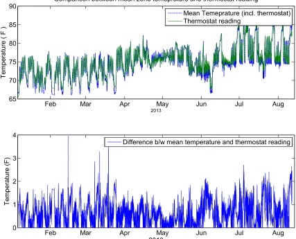
3.14 All the temperature measurements from different locations in suite 210. 43 3.15 Thermostat vs mean temperature . . . 44

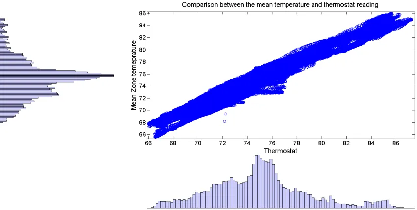
3.16 Scatter plot between the mean temperature and thermostat reading . 45 3.17 All temperatures Q-Q plot . . . 46

3.18 Bland-Altman plots for all 6 sensors . . . 46

(17)

3.20 Training data for Building 101 . . . 50

3.21 Predicted and actual zone temperature . . . 51

3.22 Input uncertainty analysis for Building 101 . . . 52

3.23 Model accuracy sensitivity coefficients for Building 101 . . . 53

4.1 Recursive partitioning and regression trees . . . 60

5.1 Rule-based vs. DR-Advisor . . . 66

5.2 DR-Advisor Architecture . . . 67

5.3 Demand Response Time line and Baseline Prediction. . . 69

5.4 Demand Response Strategy Evaluation. . . 71

5.5 Example training data for DR-Advisor . . . 73

5.6 Accuracy of auto-regressive trees for temperature predictions. . . 76

5.7 Mixed order regression tree. . . 77

5.8 Separation of variables . . . 79

5.9 DR-synthesis algorithm overview . . . 81

5.10 Linear model assumption at the leaves. The top figure shows the com-parison between fitted values and ground truth values of power con-sumption for one of the leafs in the power concon-sumption prediction tree. The bottom figure shows the residual error between fitted and actual power consumption values for all the leaf nodes of the tree. . . 82

5.11 Separation of variables accuracy. . . 83

5.12 Screenshot of the DR-Advisor MATLAB based GUI. . . 85

5.13 DR-Advisor Workflow . . . 86

5.14 DRAdvisor model identification tab . . . 87

5.15 Building 101 and DoE commercial reference building. . . 88

5.16 Penn campus buildings . . . 88

5.17 Model validation for the clinical research building at Penn. . . 89

5.18 Model validation for Building 101 . . . 91

5.19 Resubstitution error in random forest . . . 92

5.20 Predictor variables (feature) importance in the random forest ensemble. 92 5.21 Training data for the ASHRAE Great Energy Predictor Shootout Chal-lenge.. . . 94

5.22 Whole building electricity (WBE) training data . . . 95

5.23 Resubstitution error is shown for the number of trees in the random forest method. . . 96

5.24 Comparison between predicted and ground truth values for WBE for the testing data.. . . 97

(18)

5.27 DR synthesis using the mbCRT algorithm for July 17, 2013. A

cur-tailemnt of 380kW is sustained during the DR event period. . . 101

5.28 Optimal DR strategy as determined by the mbCRT algorithm. . . 102

5.29 The mbCRT algorithm maintains the zone temperatures within the

specified comfort bounds during the DR event. . . 102

5.30 Zoomed in view of the DR synthesis showing how the mbCRT algo-rithm selects the appropriate linear model for each time-step based on

the forecast of the disturbances. . . 103

6.1 Attributes at leaf nodes . . . 108

6.2 Attributes defined at each leaf node of the tree in a random forest.. . 109

6.3 Comparison between predicted and actual power consumption of the

building over the test-set. . . 110

(19)

Chapter 1 Introduction

1.1 Motivation

In 2013, a report by the U.S. National Climate Assessment provided evidence that the most recent decade was the nations warmest on record [Melillo et al. 2014] and experts predict that temperatures are only going to rise. In fact, the year 2015 is likely to become the hottest year on record since the beginning of weather recording in 1880 [NOAA 2015]. Heat waves in summer and polar vortexes in winter are growing longer and pose increasing challenges to an already over-stressed electric grid. With the increasing penetration of renewable generation, the electricity grid is experiencing a shift from predictable and dispatchable electricity generation to variable and non-dispatchable generation. This adds another level of uncertainty and volatility to the electricity grid as the relative proportion of variable generation vs. traditional dis-patchable generation increases. The volatility due to the mismatch between electricity generation and supply further leads to volatility in the wholesale price of electricity. An example of such price volatility is shown in Figure 1.1 where the fluctuations in electricity price from a single day in January, 2014th are shown for the PJM inde-pendent system operator (ISO); one of the largest grid operators in the world. In another example the polar vortex triggered extreme weather events in the U.S. in January 2014, which caused many electricity customers to experience increased costs. Parts of the PJM electricity grid experienced a 86 fold increase in the price of electric-ity from $31/MW h to $2,680/MW h in a matter of a few minutes [Michael J. Kormos 2014]. Similarly, the summer price spiked 32 fold from an average of $25/MW h to $800/MW h in July of 2015 as shown in Figure 1.2. Such events show how unfore-seen and uncontrollable circumstances can greatly affect electricity prices that impact (independent system operators) ISOs, suppliers, and customers. Energy industry ex-perts are now considering the concept that extreme weather, more renewables and resulting electricity price volatility, could become the new norm.

(20)

Figure 1.1: Volatility in real-time electricity prices in the PJM ISO from January 2014.

is a prominent component of growing efforts to supply affordable, reliable and clean electric power; most utilities and system operators are increasingly turning to demand response as a cost effective and environmentally responsible way to serve peak load. The potential demand response resource contribution from all U.S. demand response programs is estimated to be nearly 72,000 megawatts, or about 9.2 percent of U.S. peak demand [Commission et al. 2012] making DR the largest virtual generator in the U.S. national grid. The revenue to end-users from DR markets with PJM ISO alone is about $700 million [Interconnection 2014]. A recent report [Research 2015] estimates that the global commercial and industrial (C&I) DR revenue is expected to reach nearly $40 billion from 2014 through 2023.

(21)

Figure 1.2: Steep increase of 32 fold in the wholesale electricity prices in July 2015.

payments designed to induce lower electricity use at times of high market prices or when system reliability is jeopardized. Demand response programs are designed to elicit changes in customers electric usage patterns. Many DR programs vary the price of electricity over time to motivate customers to change their consumption patterns; this approach is termed price-based demand response. Other DR programs reward customers for reducing their electric loads upon request or for giving the electric util-ity some level of direct control over the customers electricutil-ity-using equipment. These are termed incentive or event-based demand response.

(22)

Figure 1.3: Electricity and natural gas consumption breakdown for commercial buildings in the United States.

programs to help manage their electricity costs. Such customers are increasingly looking to DR programs to help manage their electric utility costs.

However, to take advantage of real-time pricing and DR programs, the C/I/I

consumers must monitor electricity prices and be flexible in the ways they choose to use electricity.

1.1.1 Modeling challenges for cyber-physical energy systems

Energy systems are experiencing a gradual but substantial change in moving away from being non-interactive and manually-controlled systems to utilizing tight inte-gration of both cyber (computation, communications, and control) and physical rep-resentations guided by first principles, at all scales and levels. These cyber-physical energy systems are characterized by multiple coordinated controllers (spread across a large building or a campus), the inter-working of different energy types (natural gas, electricity, steam & hot water), the interaction with real-time energy pricing markets, integration of renewable energy sources (solar, wind and on-site genera-tion), automated and grid-friendly building operations, knowledge about the system operations due to sensors and data analytics, information technology and security challenges.

(23)

system. Consequently, the modeling effort should be tailored to suit the needs of a given application.

Control-oriented predictive models of an energy system’s dynamics and energy consumption, are needed for understanding and improving the overall energy effi-ciency and operating costs. Combining different aspects like physical infrastructure, communication systems, electricity markets, operations and people leads to a hetero-geneous system that is complex to model. The complexity arises due to the interaction between a large number of subsystems and their very different nature with respect to physical dynamics, uncertain behavior, timing and size. System identification techniques are usually used to identify parameters of a physics based white-box or grey-box model which attempt to model the system behavior. The preference for building first principles based models, arises due to the fact that the parameters of these models have a physical meaning and that the model structure is suitable for control synthesis. However, the major barrier in modeling energy systems with white box and grey box approaches, is the user expertise, time, and associated high costs required to develop a mathematical model that accurately reflects reality. This in-cludes the installation cost of retrofitting the building with additional sensors, costs related to the training of the engineering, commissioning and service personnel to im-plement model-based control and the cost of the necessary engineering effort required for constructing a model.

In the context of buildings and their energy systems, an alternative to traditional rule-based building control is model-based control. In rule-based control the opera-tion of the mechanical and electrical systems is purely “reactive” i.e. it is continuously adjusted in response to weather variations and the thermal load due to building occu-pants. With a reasonably accurate forecast of future weather and building operating conditions, dynamical models can be used to predict the energy needs of the building over a prediction horizon. Once such a model is made available, it can be used to design an optimal controller that balances comfort and energy usage. To achieve building-level energy-optimality, the model should be able to capture the interaction between physically connected spaces in the building, occupancy schedules, and the state and control input constraints. Such model-based control techniques for build-ing operations require high-fidelity white-box or grey-box models of the buildbuild-ing’s thermal envelope and equipment.

(24)

fac-Figure 1.4: Electricity and natural gas consumption breakdown for commercial buildings in the United States.

tors: such as occupancy level, internal heat generation from lighting, and computers. These quantities are highly time-varying and therefore the dynamics of the building and, consequently, parameters of the mathematical model describing the dynamics of the buildings are constantly changing with time.

(25)

Furthermore, to attain energy efficiency, control algorithms need to be tailored to the physical properties of the building at hand. Successful experience with one building is usually not repeatable on other buildings, until the domain expert has conducted a few rounds of physical experiments with the new buildings.

The alternative is to use black-box, or completely data-driven modeling approaches, to obtain a realization of the system’s input-output behavior. The primary advantage of using data-driven methods is that it has the potential to eliminate the time and effort required to build white and grey box building models. Listening to real-time data, from existing systems and interfaces, is far cheaper than unleashing hoards of on-site engineers to physically measure and model the building. The key is to identify the key dynamics that help describe the building and its behavior at the macro level. Development of data-driven models for long-term energy consumption prediction, building equipment modeling and occupancy modeling by applying machine learning algorithms such as neural networks and regression has been investigated by several researchers [Edwards et al. 2012, Kialashaki and Reisel 2013b, Vaghefi et al. 2014,

Yin et al. 2012, Hong et al. 2013]. However, the benefit obtained from the simplicity of model capture comes at the cost of having non-physical parameters and incapacity for control design and synthesis.

Improved building technology and better sensing is fundamentally redefining the opportunities around smart buildings. Decisions on how best to optimize todays building operations are becoming so complex, so conflicting and so continuous that advanced algorithms must play a role. But with complexity, comes opportunity. As complex as it can be, it is always best to start simple and learn by listening. Un-precedented amounts of data from millions of smart meters and thermostats installed in recent years has opened the door for systems engineers and data scientists to an-alyze and use the insights that data can provide, about the dynamics and power consumption patterns of these systems. The challenge now, with using data-driven approaches, is to close the loop for real-time control and decision making in large scale cyber-physical energy systems. Furthermore, providing a technological solution alone is not enough, the solution must provide interpretability and guidance to the system’s facilities managers and domain experts.

1.2 Research Goals

The focus of this research is to use data-driven approaches for making model capture easy and efficient for cyber-physical energy systems. The cost and time prohibitive process of grey/white box model capture can be made simpler or eliminated altogether by: (a) reducing the need for sensor retrofits required for estimating the parameters of first principle based models, and (b) relying more on readily available data rather than domain experts for building control-oriented models.

(26)

com-Figure 1.5: Comparison of modeling methods for cyber-physical energy systems.

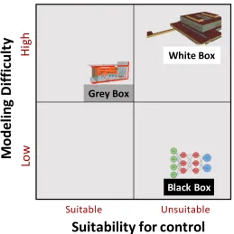
plexity and their suitability for model based control. As discussed in Section 1.1.1, white box models are extremely cost and time prohibitive to learn and are largely unsuitable for model based control. Therefore, they are in the top right of the com-parison chart of Figure 1.5. Although, grey-box models are suitable for model-based control design of buildings they are still expensive to learn and pose significant dif-ficulties in model capture both in terms of modeling time and modeling cost due to additional sensors and domain experts. Lastly, on the bottom right of the comparison chart we have, black-box models. While black-box models are easier to learn, since they only require historical data and the modeling process can be automated, they are not well suited for model-based control design and synthesis. Their use, in the con-text of buildings and other cyber-physical energy systems is limited to only prediction. Consequently, the goal of this thesis is to devise methods which can make grey-box modeling much easier and low-cost and make black-box modeling more suitable for model-based control synthesis.

Specifically, this thesis answers the following questions:,

1. Low-cost building model capture: Using a temporary sensor deployment,

(a) Can we determine the benefit obtained from adding additional sensors to a building, on model accuracy and thus, on control performance of a model-based controller ?

(27)

2. Data-driven modeling and control for demand response:

(a) Can we develop data-driven methods for building model capture which are suitable for control synthesis ?

(b) Can we provide interpretable energy consumption models for buildings ?

Small and medium sized buildings constitute more than 90% of the commer-cial buildings stock in the Unites States, but only about 10% of such buildings are equipped with a building automation system [Katipamula et al. 2012] and enough sensors to learn first principles based models. The sheer cost of building energy modeling makes it something that is primarily done by researchers and for large projects [Z´aˇcekov´a et al. 2014ˇ ]. It is not a cost that the retrofit market or most use cases would absorb in the foreseeable future without drastic reductions in the cost of having cheaper, yet accurate model generation. It is the main hurdle towards adopt-ing model-based control design approaches for cyber-physical energy systems and the goal of this thesis is to remove this hurdle.

The goal of this dissertation is to develop data-driven methods of model capture and control for cyber-physical energy systems, in particular for commercial buildings which are subject to time varying electricity prices and demand response tariffs by the electric utility companies. The proposed methods are integrated into ready to use and deployable tools. Several comprehensive case studies in data-driven building model-ing, model-based design and demand response for buildings have been conducted to show the potential of the approach. The challenges associated with answering each research question are briefly described below:

1.2.1 Low-cost building model capture

Learning mathematical models of buildings from sensor data has a fundamental prop-erty that the model can only be as accurate and reliable as the data on which it was trained. Any measurement exhibits some difference between the measured value and the true value and, therefore, has an associated uncertainty. Non-uniform measure-ment conditions, limited sensor calibration, the amount of sensor data and the amount of excitation of the plant make the measurements in the field vulnerable to errors.

A major challenge to the use of models for buildings controls lies in understanding the impact of uncertainty in the model structure, the estimation algorithm, and the quality of the training data. It is known that the quality of the training data, characterized by uncertainty, depends on factors such as the accuracy of sensors, sensor placement and density, and the assumption that air is well mixed. It is intuitive to assume that installing additional sensors to obtain higher quality training data should result in more accurate models, which will further result in better performance of a model-based controller (e.g., Model Predictive Control (MPC)).

(28)

the least sensor cost. One approach to obtaining the necessary data for generating a high-fidelity building model involves installing low-cost temporary wireless sensors and measuring the necessary model inputs and outputs for a sufficient period of time to enable training and testing of the building model.

However an understanding of the cost-benefit associated with adding additional sensors to a building is either limited or missing altogether.

1.2.2 Data-driven control oriented modeling for demand

re-sponse

On the surface demand response may seem simple. Reduce your power when asked to and get paid. However, in practice, one of the biggest challenges with end-user demand response for large scale consumers of electricity is the following: Upon re-ceiving the notification for a DR event, what actions must the end-user take in order to achieve an adequate and a sustained DR curtailment? This is a hard question to answer because of the following reasons:

1. Modeling complexity and heterogeneity: Unlike the automobile or the

air-craft industry, each building is designed and used in a different way and there-fore, it must be uniquely modeled. Learning predictive models of building’s dynamics using first principles based approaches (e.g. with EnergyPlus [ Craw-ley et al. 2001]) is very cost and time prohibitive and requires retrofitting the building with several sensors [Sturzenegger et al. 2015];

2. Limitations of rule-based DR: The building’s operating conditions,

inter-nal thermal disturbances and environmental conditions must all be taken into account to make appropriate DR control decisions, which is not possible with using rule-based and pre-determined DR strategies since they do not account for the state of the building but are instead based on best practices and rules of thumb.

3. Control complexity and scalability: Upon receiving a notification for a

DR event, the building’s facilities manager must determine an appropriate DR strategy to achieve the required load curtailment. These control strate-gies can include adjusting zone temperature set-points, supply air temperature and chilled water temperature set-point, dimming or turning off lights, decreas-ing duct static pressure set-points and restrictdecreas-ing the supply fan operation etc. In a large building, it is difficult to asses the effect of one control action on other sub-systems and on the building’s overall power consumption because the building sub-systems are tightly coupled.

4. Interpretability of modeling and control: Predictive models for buildings,

(29)

inter-preted by human experts and facilities managers in the field. Therefore, the required solution must be transparent, human centric and highly interpretable.

Regardless of the specific DR program, upon receiving a notification for a demand response event, the building’s facilities manager must determine an appropriate or op-timal control strategy to achieve the required power curtailment level. These control strategies can include adjusting zone temperature set-points, increasing supply air temperature and chilled water temperature set-point, dimming or turning off lights, decreasing duct static pressure set-points and restricting the supply fan operation etc. In a large building, it is difficult to asses the effect of one control action on other sub-systems and on the building’s overall power consumption because the building sub-systems are tightly coupled. Moreover, the performance of any DR strategy will vary due to the outside weather conditions, during the DR event.

The goal with data-driven demand response is to make the best of both worlds; i.e. keep the simplicity of rule based approaches and the predictive capability of model based strategies, but without the expense of first principle or grey-box model development.

1.3 Contributions

The contributions of this dissertation, are summarized below:

• Sensor data quality vs model accuracy: We have developed, Model-IQ, a

method to quantify how the quality of the data from sensors affects the accuracy of a building model. This is based upon our input uncertainty propagation and analysis algorithm. This was published in [Behl et al. 2014b]

• Model accuracy vs control performance: Using Model-IQ we empirically

establish the effect of model accuracy on the performance of a model-based closed-loop controller for buildings, such as mode-predictive control.

• Sensor placement and density: Using non-parametric statistical methods

and temporary sensors, we have a developed method to quantify the bias in a sensor measurement due to the location and density of sensors with applications to determine the near optimal sensor positions. This work has been published in [Behl et al. 2014a]

• DR Baseline Prediction: We demonstrate the benefit of using regression

(30)

• DR Strategy Evaluation: We present an approach for building auto-regressive trees and apply it for demand response strategy evaluation. Our models takes into account the state of the building and weather forecasts to help choose the best DR strategy among several pre-determined strategies.

• DR Control Synthesis: We introduce a novel model based control with

re-gression trees (mbCRT) algorithm to enable control with rere-gression trees use it for real-time DR synthesis. Using the mbCRT algorithm, we can optimally trade off thermal comfort inside the building against the amount of load curtailment. While regression trees are a popular choice for prediction based models, this is the first time regression tree based algorithms have been used for controller synthesis with applications in demand response.

• DR-Advisor (Demand Response-Advisor), Our methods have been

inte-grated into a MATLAB based tool called DR-Advisor, which acts as a recom-mender system for the building’s facilities manager and provides the power con-sumption prediction and control actions for meeting the required load curtail-ment and maximizing the economic reward. Using historical meter and weather data along with set-point and schedule information, DR-Advisor builds a family of interpretable regression trees to learn non-parametric data-driven models for predicting the power consumption of the building. This work has resulted in a series of publications [Behl et al. 2016, Behl and Mangharam 2015a,b, Behl et al. 2015, Behl and Mangharam 2015c].

• Energy analytics with regression trees: We present a methodology to

preserve interpretability of ensemble regression trees based methods and use the ensembles for providing energy analytics, beyond demand response, to the facilities manager based on data.

1.4 Organization

The remaining chapters of this dissertation are organized as follows:

Chapter 2: Building modeling with first principles

We start by describing the different types of modeling methods used for building modeling, namely white-box, grey-box and black-box modeling. We then present in detail each of the modeling methods and the limitations and challenges associated with each method. We then present the basics of a grey-box modeling method called the RC model of the heat transfer and use it to create a state-space dynamical model of a single zone. This chapter provides the reader with the background of building energy modeling and describes why the modeling techniques are time consuming and expensive.

(31)

This chapter uses the modeling principles described in chapter 2 to address the first research goal of this dissertation i.e. how can we lower the cost of additional sensors required to tune grey-box building models. We begin this chapter with a description of the input uncertainty analysis algorithm in Section3.2. Given a model structure and a input-output data-set, the algorithm analyzes the trade-off between sensor data quality and model accuracy. This is the basis of the Model-IQ toolbox. We next, describe how we can use empirical methods to evaluate the trade-off between model accuracy and the performance of a closed loop model based controller such as model predictive control in Section 3.4. Section3.5 then describes a non-parametric statistical approach for computing sensor bias and for sensor placement and density insights. We present a comprehensive case study in Section 3.6 using data from a real office building and show how Model-IQ can be used for understanding sensor deployment trade-offs for grey-box modeling of this building. We conclude the chapter with a summary of related work in Section 3.7 and a short discussion in Section 3.8

Chapter 4: Data-driven modeling with regression trees

Chapter 4 presents an overview of data-driven modeling using regression tree based algorithms. In this chapter, we formally introduce the principles of data-driven approaches and provide illustrative examples of how regression trees are constructed. The methods described in this chapter form the basis of the data-driven modeling and control approaches described later in Chapter 5. In this chapter we cover the seminal algorithm to construct regression trees, CART, followed by brief descriptions about extensions of that algorithm in the form of cross-validated trees, boosted regression trees, random forests and the M5 model based regression trees.

Chapter 5: Data-Driven Modeling and Control for DR

This chapter covers the methods which fulfill the second research goal of this dissertation i.e. making data-driven model suitable for close loop control synthesis and apply them to the problem demand response of cyber-physical energy systems. We first present a description of the three challenging problems in demand response in Section 5.1. This is followed by Section 5.2, which presents a description of how the regression trees algorithms presented in Chapter 4 can be utilized to solve the DR challenges. Section 5.3, presents a new algorithm to perform real-time control with regression trees and applied to the DR synthesis problem. Section 5.4 makes a compelling case for regression trees being a suitable choice of data-driven models for real-time DR. Section 5.5 describes the MATLAB based DR-Advisor toolbox. Section5.6 presents a comprehensive case study with DR-Advisor on data from 8 real buildings on Penn’s campus, a large office building, a virtual test-best and evaluation of the tool on bench-marking data from ASHRAE’s energy prediction competition. In Section 5.7, a detailed survey of related work has been presented. We conclude this chapter in Section 5.8 with a summary of our results.

(32)

This chapter describes how the regression trees based models described in Chap-ters4and5can also be used for energy analytics in order to assist a facilities manager understand more about the energy usage of his building/campus. In this chapter, we describe the extension to regression trees which allows us to build data-structures which can be searched to provide answers to open ended queries about the system from the facilities manager. At the core of the chapter is the idea of converting the regression tree models into a searchable and interpretable knowledge database. We demonstrate this idea using data from a real building on Penn’s campus.

(33)

Chapter 2 Building modeling with first

principles

For the simulation and control of buildings, models of appropriate accuracy and complexity are essential. A variety of simulation tools that have been developed for building energy analysis, simulation, control design and building design automation. In this chapter, we present an overview of different techniques for building modeling using first principles of physics and heat transfer. We will present examples and describe tools which are often used for building such models.

The main objective of an HVAC system for air temperature control is to reject disturbances due to outside weather condition and internal heat gain/loss caused by occupants, lighting and plug-in appliances.

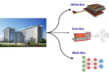
Therefore, the building model must accurately capture the thermal response of the building to the different disturbances and due to the hVAC control. Building models for cyber-physical energy systems can be broadly classified into three categories as shown in Figure 2.1:

1. White-box models are based on the laws of physics and permit accurate and microscopic modeling of the building system. High fidelity building simulation programs like EnergyPlus and TRNSYS [Crawley et al. 2008] fall into this category. Although such models provide a high degree of accuracy they are unsuitable for control design due to their high level of complexity and a large number of parameters. Furthermore, the process of constructing the model and tuning the parameters with limited data is very time consuming and not cost effective.

2. Black-box models are not based on physical behaviors of the system but rely on the available data to identify the model structure. These models are often purely statistical and have a simple structure.

(34)

Figure 2.1: Modeling categories for cyber-physical energy systems

and the available data is used to estimate the values of the model parame-ters. These models are suitable for model-based control design and rely on first principles based modeling.

We now describe white-box and grey-box modeling methods for buildings in detail:

2.1 White-box modeling

(35)

Figure 2.2: White-box building modeling approach for buildings.

match the measured data from the building. This tuning process is highly subjective and repeatable across neither modelers nor software packages.

Furthermore, tuning such a software model also requires that the building be retrofitted with enough sensors which can generate high resolution spatial and tem-poral data which can be used to tune the parameters of the building model. The two most popular softwares for building energy modeling are EnergyPlus and TRNSYS. We breifly describe them next.

2.1.1 EnergyPlus

(36)

in-put, and output files including hourly or sub-hourly environmental conditions, and standard and user definable reports. It leverages heat balance-based techniques for building thermal loads that allow for simultaneous calculation of radiant and con-vective effects at both interior and exterior surface during each time step. Transient heat conduction through building elements such as walls, roofs, floors, etc. using con-duction transfer functions are also supported. EneryPlus also features combined heat and mass transfer model that accounts for moisture absorption/desorption. Thermal comfort models based on activity, inside dry bulb, and humidity as well as anisotropic sky model for improved calculation of diffuse solar on tilted surfaces are available. Detailed and advanced fenestration calculations in EnergyPlus includes controllable window blinds, electrochromic glazings, layer-by-layer heat balances that allow proper assignment of solar energy absorbed by window panes, and a performance library for numerous commercially available windows. Daylighting controls including interior illuminance calculations, glare simulation and control, luminaire controls, and the effect of reduced artificial lighting on heating and cooling are the other features sup-ported by EnergyPlus. EnergyPlus is regarded as a very detailed and high-fidelity whole building simulation tool. This makes EnergyPlus a good choice if the objective of the study is to analyze and compare the effects of some building features. On the other hand, being a very detailed modeling tool, EnergyPlus is not a program of choice if the task is model-based control design.

2.1.2 TRNSYS

(37)

Figure 2.3: Grey-box building modeling approach for buildings.

energy modeling software. However, it would still require one to build the EnergyPlus model first from the building design, construction and operation information. Such approaches are also limited in their impact on reducing the cost of additional sensor retrofits required to tune the models.

2.2 Grey-box models

The grey-box building modeling approach is very similar to the white-box modeling approach expect for two key differences:

• Firstly, the domain expert or the building modeler does not need to consider the design , construction details and operation of the building is as much detail as the white box model. Certain details are aggregated or ’lumped’ together to reduce model complexity; and

• Secondly, instead of using a software simulation to add parameter values, in grey-box modeling, the model structure itself is built from scratch, using first principles, by the domain expert as shown in Figure 2.3.

(38)

Figure 2.4: RC lumped-parameter model representation for a thermal zone obtained from information about the zone geometry and usage.

The American Society of Heating, Refrigerating, and Air Conditioning (ASHRAE) has established extensive methodologies for calculation of heating and cooling loads in [ASHRAE 2009]. Such methodologies involve heat balance analysis. It is a straight-forward physics-based and comprehensive methodology that involves calculating a node-to-node heat balance of a room through consideration of conductive, convective, and radiative heat transfer mechanisms, a node can either be wall or air in the room. A commonly used grey-box representation of the thermal response of a building due, which uses this ASHRAE methodology, is based on a lumped parameter Resistive-Capacitative (RC) network. This approach for modeling buildings represents has been used widely, e.g. in [Braun and Chaturvedi 2002, McKinley and Alleyne 2008,

Dewson et al. 1993]. Figure 2.4 shows an example of such a model for a single zone, as used in [Braun and Chaturvedi 2002]. In this representation, the central node of the RC network represents the zone temperature Tz(◦C). The geometry of the zone

is divided into different kinds of surfaces, each of which is modeled using a ‘lumped-parameter’ branch of the network. For instance, all the external walls of the zone are lumped into a single wall with 3R2C (3 resistances and 2 capacitance) parameters. The same process is applied to the ceiling, the floor and the internal (or adjacent) walls of the zone. The zone is subject to several (heat) disturbances which are applied at different nodes in the network in the following manner:

(a) solar irradiation on the external wall ˙Qsol,e(W) and the ceiling ˙Qsol,c(W) is applied

on the exterior node of the lumped wall,

(b) incident solar radiation transmitted through the windows ˙Qsolt(W) is assumed to

be absorbed by the internal and adjacent walls,

(c) radiative internal heat gain ˙Qrad(W) which is distributed with an even flux to

(39)

Table 2.1: List of parameters

U?o convection coefficient between the wall and outside air

U?w conduction coefficient of the wall

U?i convection coefficient between the wall and zone air

Uwin conduction coefficient of the window

C?? thermal capacitance of the wall

Cz thermal capacity of zone zi

g: floor; e: external wall; c: ceiling; i: internal wall

(d) the convective internal heat gain ˙Qconv(W) and the sensible cooling rate ˙Qsens(W)

is applied directly to the zone air,

(e) the zone is also subject to heat gains due to the ambient temperature Ta(◦C),

ground temperatureTg(◦C) and temperatures in other zones which are accounted

for by adding boundary condition nodes to each branch of the network.

The list of all parameters in the model and their descriptions is given in Table 2.1. Given this model, the nodal equations for the lumped external wall and the ceiling network are:

CeoT˙eo(t) =Ueo(Ta(t)−Teo(t)) +Uew(Tei(t)−Teo(t)) + ˙Qsol,e(t)

CeiT˙ei(t) =Uew(Teo(t)−Tei(t)) +Uei(Tz(t)−Tei(t)) + ˙Qrad,e(t)

CcoT˙co(t) =Uco(Ta(t)−Tco(t)) +Ucw(Tci(t)−Tco(t)) + ˙Qsol,c(t)

CciT˙ci(t) =Ucw(Tco(t)−Tci(t)) +Uci(Tz(t)−Tci(t)) + ˙Qrad,c(t)

(2.1)

CeoT˙eo(t) = Ueo(Ta(t)−Teo(t)) +Uew(Tei(t)−Teo(t))

+ ˙Qsol,e(t) (2.2a)

CeiT˙ei(t) = Uew(Teo(t)−Tei(t)) +Uei(Tz(t)−Tei(t))

+ ˙Qrad,e(t) (2.2b)

CcoT˙co(t) = Uco(Ta(t)−Tco(t)) +Ucw(Tci(t)−Tco(t))

+ ˙Qsol,c(t) (2.2c)

CciT˙ci(t) = Ucw(Tco(t)−Tci(t)) +Uci(Tz(t)−Tci(t))

+ ˙Qrad,c(t) (2.2d)

Similarly, one can write the equations for the dynamics of the nodes of the floor and internal wall network. The law of conservation of energy gives us the following heat balance equation for zone

CzT˙z(t) = Uei(Tei(t)−Tz(t)) +Uci(Tci(t)−Tz(t))

+Uii(Tii(t)−Tz(t)) +Ugi(Tgi(t)−Tz(t))

(40)

Differential equations in 2.1 and 2.3 can be combined to give a state space model of the system. Define x= [Teo, Tei, Tco, Tci, Tgo, Tgi, Tio, Tii, Tz]T to be the state vector

of all node temperatures. The input uis a vector of all the inputs to the systems, i.e.

u= [Ta, Tg, Ti,Q˙sol,e,Q˙sol,c,Q˙rad,e,Q˙rad,c,Q˙rad,g,Q˙solt,

˙

Qconv,Q˙sens]T. The control input to the zone is the sensible cooling rate ˙Qsens. The

cooling rate can be controlled by changing the mass flow rate of cold air which enters the zone (in case of cooling) or by changing the set point of the supply air temperature. The rest of the inputs are disturbances to the zone or non-manipulated inputs. The elements of the system matrices depend nonlinearly on the U and C parameters. Let us consider θ = [Ueo, Uew, Uei, . . . Cio, Cii]T as a vector of all the parameters of

the model. Then the state space equations have the following representation which emphasizes the parameterization of the system matrices.

˙

x(t) =Aθx(t) +Bθu(t)

y(t) = Cθx(t) +Dθu(t)

(2.4)

The output matrix Cθ and the feed-forward matrix Dθ depend on the outputs of

interest. For instance, if the output of the model is the zone temperature then Cθ =

[0,0, . . . ,0,1], which is a row vector with all entries equal to zero except the last entry corresponding to the zone temperature Tz equal to one. In this case Dθ = 0, the null

matrix.

This model structure is based on the underlying assumption that the air inside the zone is well mixed and hence it can be represented by a single node. Further-more, only one-dimensional heat transfer is assumed for the walls and there is no lateral temperature difference. The parameters of the model are assumed to be time invariant.

2.2.1 Parameter Estimation (Model Training)

We discretize the continuous-time model in equation 2.4 with the measurement sam-pling time to obtain a discrete-time state space model:

x(k+ 1) = ˆAθx(k) + ˆBθu(k)

y(k) = ˆCθx(k) + ˆDθu(k)

(2.5)

The goal of parameter estimation is to obtain estimates of the parameter vectorθ

of the model from input-output time series measurement data. The parameter search space is constrained both above and below by θl ≤ θ ≤ θu. For a given parameter

vectorθ, the model, given by equation2.5, can be used to generate a time series of the zone air temperatureTzθ using the measured time series data for the inputsu(k). The

subscript θ denotes that the temperature value Tzθ is the predicted value using the

model with parametersθand the inputsu. This model generated time seriesTzθ may

(41)

Tzm, and the difference between the two is quantified by a statistical metric. The

metric usually chosen is the sum of the squares of the differences between the two time series. The parameter estimation problem is to find the parameters θ∗, subject to θl ≤ θ ≤ θu, which result in the least square error between the predicted and the

measured temperature values, i.e.

θ∗ = arg min

θl≤θ≤θu

PN

k=1(Tzm(k)−Tzθ(k))

2 _(2.6)

where the summation is over the N data points of the input-output time series under investigation.

The least square optimization of equation 2.6 is a constrained minimization of a non-linear objective. It is numerically solved using a trust region reflective algo-rithm [Coleman and Li 1996] such as the Levenberg-Marquardt [Mor´e 1978] algorithm. A well known problem with non-linear search algorithms is the problem of the solution getting stuck at a local minima. It is desirable that the initial parameter estimates

θ0 are as close as practicable to their (unknown) optimal (true) values. The initial values of the parameters can be estimated from the details of the constructions and materials used for the building. Generally speaking, the further the initial guess of the parameters is away from the true values, the bigger the search region is for the optimization. As search region grows, it becomes more likely that the estimation process will converge to a local optimum.

2.3 Concluding remarks

(42)

Chapter 3 Low-Cost Building Model Capture

One of the biggest challenges in the domain of cyber-physical energy systems is in ac-curately capturing the dynamics of the underlying physical system. In the context of buildings, the modeling difficulty arises due to the fact that each building is designed and used in a different way and therefore, it has to be uniquely modeled. Further-more, each building system consists of a large number of interconnected subsystems which interact in a complex manner and are subjected to time varying environmental conditions.

Control-oriented models are needed to enable optimal control in buildings. Models for building load requirements and temperature dynamics are particularly important and often the existing sensor measurements available from the building heating ven-tilation and air conditioning (HVAC) system are not sufficient for use in training and testing a model. Learning mathematical models of buildings from sensor data has a fundamental property that the model can only be as accurate and reliable as the data on which it was trained. Any measurement exhibits some difference between the measured value and the true value and, therefore, has an associated uncertainty. Non-uniform measurement conditions, limited sensor calibration, the amount of sen-sor data and the amount of excitation of the plant make the measurements in the field vulnerable to errors. With appropriate understanding of the sources of errors and their effect on the operating cost of the controller, the errors associated with some of these sources can be minimized. In the case of using sensor data for building first principles based models (e.g. grey box or white box), the goal is to provide maximum benefit, in terms of model accuracy, for the least sensor cost.

(43)

optimiza-Model-‐IQ Toolbox

•  Input Uncertainty Analysis

•  Input Sensi:vity Coeﬃcient

Inverse Model of Building

Training Data Input Streams

Parameter Es:ma:on Algorithm

Model Accuracy and MPC Cost Tradeoﬀ

Sensor density and posi:on recommenda:on

Co

nt

ro

ller

Perfo

rma

nce

Uncertainty

Figure 3.1: Model-IQ Toolbox uncertainty analysis for building controls.

tion of selected zones in commercial buildings. Therefore, there is economic value is performing an uncertainty analysis for such installations in order to better access the tradeoffs involved in sensor installation cost and building performance.

However, a major challenge to the use of models for buildings controls lies in understanding the impact of uncertainty in the model structure, the estimation algo-rithm, and the quality of the training data. It is known that the quality of the training data, characterized by uncertainty, depends on factors such as the accuracy of sen-sors, sensor placement and density, and the assumption that air is well mixed. It is intuitive to assume that installing additional sensors to obtain higher quality training data should result in more accurate models, which will further result in better perfor-mance of a model based controller (e.g. Model Predictive Control (MPC)). However an understanding of the cost-benefit associated with adding additional sensors to a building is either limited or missing altogether. The reason for this is twofold: a) It is not clear how the quality of the data from sensors affects the accuracy of a

building model. This is because data quality is only one of several factors that may affect model accuracy.

b) It is hard to analytically establish the effect of model accuracy on the performance of a model based closed-loop controller for buildings.

The goal of this work is to study the cost-benefit effect of adding temporary low cost wireless sensors to a zone to improve model accuracy and subsequently enable low-cost implementation of advanced control schemes such as Model Predictive Control (MPC) (see 3.1). We first perform an input uncertainty analysis to classify the effect of the quality of training data on the accuracy of a “grey-box” building inverse model. We show how additional sensors can affect the training data quality. We empirically evaluate the tradeoff between model accuracy and MPC performance, i.e. all things being the same, for different model accuracies how MPC performance varies.

3.1 Uncertainty in Building Modeling

(44)

algorithm and (c) the uncertainty in the training data. In this effort, we assume the first two are fixed and focus on understanding the effect of uncertainty of the training data from the building and environment sensors on the overall performance of a model-based controller for the buildings HVAC systems.

The uncertainty in training data can be characterized in two ways: bias error or random error. Biases are essentially offsets in the observations from the true values. Bias error can also be referred to as the systematic error, precision or fixed error. The bias in the sensor measurement is due to a combination of two reasons. The first reason is the sensor precision. The best corrective action in this case is to ascertain the extent of the bias (using the data-sheet or by re-calibration) and to correct the observations accordingly. The sensor may also exhibit bias due to its placement, especially if it is measuring a physical quantity which has a spatial distribution, e.g. air temperature in a zone. In this case, it is hard to detect or estimate the bias unless additional spatially distributed measurements are obtained. Random error is an error due to the unpredictable (e.g. measurement noise) and unknown extraneous conditions that can cause the sensor reading to take some random values distributed about a mean.

The density and location of sensors in a zone affects the deviation of the mea-sured value from the true value. For instance, a zone thermostat sensor placed too close to the wall, window, supply or return air duct can introduce a bias in the zone temperature measurement. A bias in the zone temperature value can lead to wastage of energy and discomfort with simple zone air control schemes like On-Off and PID control. Both the controllers aremodel-independent i.e. they only used the measure-ment of theprocess variable (which is the room temperature in this case) to compute the control signal that will either track the set-point (PID) or keep the temperature bounded around the set-point (On-Off). As we proceed to applymodel-based control

schemes for building retrofits, the bias or the uncertainty in the measured data will also influence the accuracy of the model itself which in turn affects the performance of the model based controller.

3.2 Model-IQ approach

In this section, we describe the Model-IQ approach for analyzing uncertainty propa-gation for building grey-box models. The accuracy of the grey-box building model, described in Section 2.2, depends primarily on the following three factors:

(a) The structure of the model which depends on the extent to which the model

respects the physics of the underlying physical system,

(b) The performance of the estimation algorithm. As discussed previously,

(45)

Parameter Estimation (Inverse Model Training) Prediction Error Perturb each input stream (N perturbations) Common input for evaluation Different parameters estimated for each

perturbation

(N models) (N different fits) ..

. .. . Input Data Stream

Sensible Cooling Convective Gain External Solar Radiative gain Transmitted Solar Ambient temp. Ground temp.

Figure 3.2: Overview of the Model-IQ input uncertainty analysis methodology, an offline method to confirm the influence of each training input on the accuracy of the model.

(c) The quality of the training data, which can be characterized by its

uncer-tainty.

The main premise of the input uncertainty propagation is that once the model struc-ture and the parameter algorithm are fixed, one can study the influence of the un-certainty in the training data on the accuracy of the model using virtual simulations which utilize artificial data-sets. Figure 3.2 shows an overview of the Model-IQ ap-proach. We introduce an uncertainty bias in each of the training data streams in form of bounded perturbations around the unperturbed (nominal) values. This results in the creation of artificial training data sets each of which is similar to the original unperturbed data-set except for one input data stream. For each artificial data-set, we train a new grey-box model and calculate its test error. A common test data set allows us to fairly compare the accuracy of the models in terms of their test root mean square error (RMSE). This allows us to quantify the effect of uncertainty bias in each input stream on the accuracy of the grey-box model. For the remaining part of the section we will use an example of a building modeled in TRNSYS for conducting the input uncertainty propagation analysis.