www.nat-hazards-earth-syst-sci.net/12/1671/2012/ doi:10.5194/nhess-12-1671-2012
© Author(s) 2012. CC Attribution 3.0 License.
and Earth
System Sciences
Temperature extremes in Europe: overview of their driving
atmospheric patterns
C. Andrade1,2, S. M. Leite2, and J. A. Santos2
1Instituto Polit´ecnico de Tomar, Unidade Departamental de Matem´atica e F´ısica, Estrada da Serra, Quinta do Contador,
2300-313 Tomar, Portugal
2CITAB, University of Tr´as-os-Montes e Alto Douro, 5001-801 Vila Real, Portugal
Correspondence to: C. Andrade ([email protected])
Received: 27 February 2012 – Revised: 24 April 2012 – Accepted: 30 April 2012 – Published: 24 May 2012
Abstract. As temperature extremes have a deep impact on environment, hydrology, agriculture, society and economy, the analysis of the mechanisms underlying their occurrence, including their relationships with the large-scale atmospheric circulation, is particularly pertinent and is discussed here for Europe and in the period 1961–2010 (50 yr). For this aim, a canonical correlation analysis, coupled with a principal com-ponent analysis (BPCCA), is applied between the monthly mean sea level pressure fields, defined within a large Euro-Atlantic sector, and the monthly occurrences of two temper-ature extreme indices (TN10p – cold nights and TX90p – warm days) in Europe. Each co-variability mode represents a large-scale forcing on the occurrence of temperature ex-tremes. North Atlantic Oscillation-like patterns and strong anomalies in the atmospheric flow westwards of the British Isles are leading couplings between large-scale atmospheric circulation and winter, spring and autumn occurrences of both cold nights and warm days in Europe. Although sum-mer couplings depict lower coherence between warm and cold events, important atmospheric anomalies are key driving mechanisms. For a better characterization of the extremes, the main features of the statistical distributions of the abso-lute minima (TNN) and maxima (TXX) are also examined for each season. Furthermore, statistically significant down-ward (updown-ward) trends are detected in the cold night (warm day) occurrences over the period 1961–2010 throughout Eu-rope, particularly in summer, which is in clear agreement with the overall warming.
1 Introduction
Europe has been experiencing strong extreme events over the last decades, including temperature extremes, namely cold spells and heat waves. These extreme events, such as the 2003 and 2005 European heat waves (Sch¨ar et al., 2004; Trigo et al., 2005; Chase et al., 2006; Della-Marta et al., 2007; Santos et al., 2007; Luterbacher, 2010), the unusually cold and snowy/rainy winters of 2009 (central and western Europe) and 2010 (Wang et al., 2010; Andrade et al., 2011; Guirguis et al., 2011), had a great impact on many socio-economic sectors throughout Europe, including increases in the mortality rates (WHO, 2003; Milligan, 2004; Poumad`ere et al., 2005; Robine et al., 2008). Therefore, owing to the impacts temperature extremes have on human activities, wa-ter and energy supply (IPCC, 2008; Koch and V¨ogele, 2009; F¨orster and Lilliestam, 2010), agricultural resources (Ferris et al., 1998), forest fires (Pereira et al., 2005; Moriondo et al., 2006), and economy in general, their understanding is of utmost relevance not only for scientists and decision-makers, but also for the whole society.
percentile-based indices have been employed, which are climate-adaptive indices, i.e. defined taking into account the actual distribution of the climate variables at each location (Peterson, 2005; Alexander et al., 2006). In particular, some indices of temperature extremes allow the assessment of the coldest (warmest) deciles of TN and TX within a given time period. In fact, the present study is mainly focused on the analysis of the 10th and 90th percentiles of the daily TN and TX: TN10p (cold nights) and TX90p (warm days), respec-tively, over the period 1961–2010 (50 yr). These temperature percentile-based indices allow the assessment of the variabil-ity in the frequencies of occurrence of the warmest (coldest) events in the selected time period. In order to properly take into account the strong temperature seasonality, the study is also primarily conducted for winter (December, January and February, DJF) and summer (June, July and August, JJA) and secondly for spring (March, April, May, MAM) and autumn (September, October, November, SON), separately.
Extreme events in Europe and in the Mediterranean basin are usually linked to specific large-scale atmospheric circu-lations in the Northern Atlantic (Xoplaki et al., 2003; Santos and Corte-Real, 2006; Rodr´ıguez-Puebla et al., 2010). As il-lustrations of this large-scale forcing, it can be mentioned the role that the anticyclonic ridges over the eastern North At-lantic play in triggering droughts and precipitation extremes over the Iberian Peninsula (Santos et al., 2008; Andrade et al., 2011; Costa et al., 2012) or heat waves in Europe (Cas-sou et al., 2005; Carril et al., 2008). Relationships between the North Atlantic Oscillation (NAO) and climate extremes have also been previously reported (e.g. Santos et al., 2007; Scaife et al., 2008). Nonetheless, the causes for the occur-rences of these events are not entirely systematized and de-serve further research, particularly bearing in mind the sus-ceptibility of Europe and the Mediterranean (Xoplaki et al., 2003; Giorgi, 2006; Diffenbaugh et al., 2007; Jones et al., 2008; Kuglitsch et al., 2010) to temperature extremes.
Along the previous lines, as climate variability in Europe is strongly influenced by the variability of the large-scale at-mospheric circulation, this study aims at understanding the links between the large-scale circulation in the Euro-Atlantic sector and the occurrences of temperature extremes in Eu-rope, in winter, summer, spring and autumn. For this purpose, multivariate statistical tools are applied in order to isolate the main modes of the co-variability between these fields, thus allowing for the detection of large-scale forcing mechanisms on the occurrence of temperature extremes in Europe. A bet-ter understanding of these driving mechanisms may hope-fully help mitigating their adverse impacts all across the con-tinent.
The study is then organized as follows: in Sect. 2 the datasets and methodologies are described; Sect. 3 includes three subsections for winter, summer and transitional sea-sons (spring and autumn): the first comprises both a pre-liminary extreme value analysis of the TNN and TXX and a trend analysis of the TN10p and TX90p, while the second
subsection is devoted to the discussion of the large-scale cou-pling modes in the TN10p and TX90p; lastly, the most rele-vant conclusions are summarized in Sect. 4.
2 Data and methodology
In the present study two datasets were used: (1) the E-OBS dataset (Haylock et al., 2008), which is a gridded obser-vational dataset produced by the EU-FP6 project ENSEM-BLES and is available at the European Climate Assessment and Dataset (ECA&D) website (http://eca.knmi.nl/), from which daily TN and TX were retrieved on a 0.25×0.25◦ latitude-longitude grid. Although the interpolation from sta-tion data to gridded values can significantly smooth extreme events (Haylock et al., 2008), this dataset still provides use-ful information on moderate temperature extremes. Further-more, it provides spatially homogeneous data on a rela-tively high spatial resolution and can also be more directly compared to climate model data than station data in forth-coming studies. (2) The National Centers for Environmental Prediction (NCEP) reanalysis dataset (Kalnay et al., 1996), which provided the monthly means of the sea level pressure (MSLP), zonal and meridional wind components at 850 hPa, air temperature at 850 hPa and total cloud cover (TCC) for the entire atmospheric column. With the exception of TCC, which is defined on a T62 Gaussian grid, all other reanalysed variables are defined on a 2.5◦latitude×2.5◦longitude grid. Temperature advections were computed using the wind and temperature fields and the approximation to the finite differ-ences numerical method. The MSLP is generally a reliable indicator of the large-scale atmospheric flow over extratrop-ical regions (e.g. Holton, 2004) and are used in the coupling analysis. As the temperature field is largely controlled by temperature transports and by diabatic terms (e.g. Holton, 2004), mostly radiation and latent heat fluxes, the patterns of the temperature advection and cloudiness are particularly meaningful when analysing the occurrence of temperature extremes. The 850 hPa level is considered here, because it is often above the boundary layer, but not too far from the surface, where the extremes actually occur. Even so, no sig-nificant changes were detected when using the 700 hPa level (not shown).
The TX90p (TN10p) is a percentile-based index that corre-sponds to the monthly number of days with daily maximum (minimum) temperature above its 90th (below its 10th) per-centile, computed for that specific calendar month over the full time period (1961–2010). Both indices are also com-monly referred to as the number of occurrences of cold nights (TN10p) or warm days (TX90p) (cf. Alexander et al., 2006), which can be considered moderate extremes. In fact, sim-ilar indices are recommended by the joint expert team of the World Meteorological Organization (WMO), under the CCI/CLIVAR/JCOMM project of the ETCCDI, despite some slight modifications in their definitions (http://cccma.seos. uvic.ca/ETCCDI/list 27 indices.shtml).
The time series of extremes can be more adequately tack-led by the extreme value theory (EVT), which has been widely applied in the fields of hydrology, meteorology and financial time series forecasting. In particular, EVT provides the statistical framework to estimate the probability of occur-rence of extreme or very rare events, including their associ-ated return periods, which can be used, e.g. in risk analysis (e.g. Wilks, 2006). The theoretical generalized extreme value distribution (GEV) was developed within the EVT frame-work and its cumulative distribution function,F (x), is given by (Coles, 2001)
F (x)=exph− 1+kx−µσ −1/ ki 1+kx−µσ >0
(1)
wherek,µ andσ are, respectively, the shape, location and scale parameters. In practice, the GEV comprises three types of theoretical distributions, according to the value of its shape parameter (Jenkinson, 1955): Gumbel (Type I;k=0), Fr´echet (Type II;k >0) and Weibull (Type III;k <0).
In the present study, the GEV was fitted to the seasonal time series of TNN and TXX at each grid point. The proba-bility distributions were determined using the maximum like-lihood estimation (MLE) at a 95 % confidence level. TheT -year return level can then be defined as the value that is ex-ceeded at an average time interval of T years. The return value can be calculated by solving the following equation (Coles, 2001):
xT =µ−
σ k " 1− −log
1− 1 T
−k#
, k6=0 (2) or
xT =µ−σlog
−log
1− 1 T
, k=0, (3)
for the Gumbel distribution. In this study, the uncertainty in the estimation of return values is relatively low, since only the 5-, 10- and 20-yr return periods were considered, which are clearly inferior to the 50-yr sample size.
Despite the valuable information that can be obtained from the analysis of TNN and TXX, the TN10p and TX90p are
more robust (percentile-based) and resistant (less outlier-influenced) indices, thus allowing a more accurate assess-ment of the variability of the temperature extremes. As a result, after a first outlook at TNN and TXX, TN10p and TX90p are considered in the subsequent multivariate statisti-cal approaches. Furthermore, in order to improve the sample sizes and, consequently, the accuracy of the results, TN10p and TX90p are analysed on a monthly basis rather than on a seasonal basis, which implies that the length of the time se-ries is of 150 months instead of 50 seasons. Aiming at identi-fying long-term changes in the occurrence of the temperature extremes, the linear trends in TN10p and TX90p were first calculated and their statistical significance was assessed by the Spearman’s rho test (non-parametric test; Wilks, 2006). This low frequency variability is likely to be a manifesta-tion of climate change, but only provides informamanifesta-tion about changes in the recent past conditions and cannot be extrapo-lated to future climatic conditions; this can only be achieved through numerical modelling of the climate system. These linear trends were removed in the upcoming analysis.
For assessing the relevant large-scale modes linked to the occurrence of warm (cold) winter, summer, spring and au-tumn days (nights), a canonical correlation analysis (CCA) on the empirical orthogonal function (EOF) spaces of the selected fields was applied. The resulting coupled modes aim to successively maximize the co-variability between a given pair of fields (MSLP vs. TN10p or MSLP vs. TX90p). The approach presented by Barnett and Preisendorfer (1987), herein called BPCCA, was followed to filter out small-scale noise in the datasets and to produce more stable patterns than the classical CCA, which is particularly apparent when the sample size is smaller than the spatial dimensionality of the field (Bretherton et al., 1992). Accordingly, only the most relevant orthogonal modes (cumulatively representing about 70 % of the temporal variance in each field) are retained for the CCA (Bretherton et al., 1992). In order to satisfy the stationarity constraints, the time series in each field (MSLP, TN10p and TX90p) were detrended prior to the application of the BPCCA; the trends in the indices are analysed sep-arately. Two distinct Euro-Atlantic sectors were considered in the BPCCA: (20◦N–70◦N; 60◦W–60◦E) for the MSLP and (30◦N–70◦N; 35◦W–35◦E) for TN10p or TX90p. The former sector is large enough so that key large-scale atmo-spheric features over the North Atlantic are properly taken into consideration.
variable above (below) 1 (−1). Differences between the pos-itive and negative composites were then computed for the zonal and meridional wind components at 850 hPa, for the temperature advection at the same isobaric level and for the TCC.
3 Results
3.1 Winter extremes
3.1.1 Extreme value analysis
The analysis of the statistical distributions of the extreme air temperatures can provide a first insight into their behaviour across Europe. This can be carried out by fitting extreme value distributions to the time series of the winter TNN and TXX at each grid point. As mentioned in the previous sec-tion, the GEV distributions (1) usually provide suitable the-oretical adjustments to these time series, enabling statisti-cal inference. The three parameters of the GEV distribution (shape, location and scale) were thus estimated (at a 95 % confidence level) at every grid point.
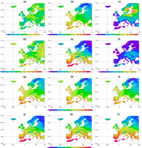
As most shape parameters tend to zero in both TNN and TXX (Fig. 1a and d), it can be concluded that the Gumbel distribution usually provides the best fits to the empirical distributions of these extremes. The distribution parameters were also used to estimate the mean and variance fields of each extreme (TNN: Fig. 1b and c; TXX: Fig. 1e and f). The means are actually very similar to the location param-eters (not shown), whereas the variances strongly resemble the squared scale parameters (not shown), suggesting some symmetry in the distributions. The mean fields essentially reflect climate-mean features, with the highest temperatures over southern Europe and the lowest temperatures over Scan-dinavia and northeastern Europe (Fig. 1b and e). The higher temperature gradients in TXX than in TNN also highlight that the thermal contrasts throughout Europe are much less pronounced at night, when the solar radiative forcing is ab-sent or negligible. The variances tend to be higher in TNN than in TXX (Fig. 1c and f), which shows that TNN presents higher variability and irregularity than TXX. Furthermore, the variance in TNN reveals very high values over the Baltic region (Fig. 1c), while the variance in TXX shows the high-est variability over eastern Europe (Fig. 1f). The high conti-nentality of these regions explains the high variances in their extreme temperatures, though the connection to large-scale patterns is explored in the next subsection. The correspond-ing temperatures associated with the 5-, 10- and 20-yr return periods (Fig. 1g–l) are computed using Eqs. (2) or (3). They give a useful measure of the exceptionality of a certain tem-perature at a given location and can be used in risk assess-ment.
As expected taking into account the European climatol-ogy, the TN10p monthly mean fields in the winter months
(Fig. 2a, b and c) show minimum negative values over north-ern, eastern and central Europe and higher values over south-ern and westsouth-ern Europe. The TX90p monthly mean fields (Fig. 2d, e and f) depict a temperature distribution quite sim-ilar to TN10p, though with substantially higher values in some regions (e.g. in northern Scandinavia their difference can be over 30◦C). This highlights the strong continentality of some European regions and their high day-night thermal contrasts. As expected, there is also a strong similarity with the mean patterns for TNN and TXX (Fig. 1b and e), as these variables are all based on the distributions of the daily TN and TX.
It is still worth mentioning the statistically significant pos-itive trend in the TX90p throughout most of Europe, particu-larly in January and February (Fig. 2j, k and l). This outcome clearly contrasts with the few and scattered significant trends for the TN10p (Fig. 2g, h and i). Therefore, while no sig-nificant and spatially coherent changes in the occurrences of cold nights are found, significant increases in the occurrences of warm days are apparent, which hints not only at the warm-ing of the European winters, but also at the significant in-crease in the occurrence of exceptionally warm days (Luter-bacher et al., 2004; Alexander et al., 2006; Haylock et al., 2008). Moreover, these results are also in clear accordance with previous results, such as those attained by Rodr´ıguez-Puebla et al. (2010) for the Iberian Peninsula, where a pos-itive trend in TX90p is reported in contrast with a negative trend in TN10p.
3.1.2 Large-scale coupling modes
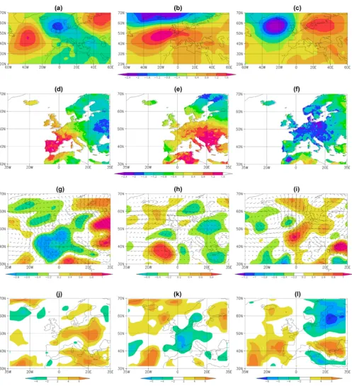
As previously stated, the BPCCA was used to assess the re-lationships between the large-scale atmospheric circulation and two extreme temperature indices in Europe, usually re-lated to the occurrence of cold nights (TN10p) and warm days (TX90p). Only the most relevant orthogonal modes were retained and used in the BPCCA: the first five PCs of the indices represent about 70 % of the total variance (69.9 % for TN10p and 72.4 % for TX90p), whilst the first three PCs of MSLP represent 71.7 % of its variance. The discussion will be focused on the first three coupled modes that present canonical correlations of 0.58, 0.35 and 0.30 for TN10p and 0.64, 0.42 and 0.30 for TX90p. Higher order coupled modes are not statistically significant and will not be considered here.
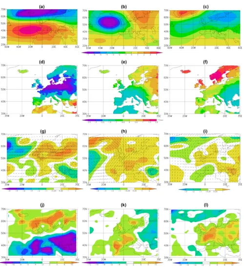
been extensively analysed (e.g. Wallace and Gutzler, 1981; Barnston and Livezey, 1987; Hurrell, 1995; Hurrell and van Loon, 1997; Pozo-V´azquez et al., 2001; Pinto and Raible, 2012). The positive phase of the NAO (anomalously strong Azores high and anomalously strong Iceland low) tends to be associated with above-average temperatures over north-ern and central Europe and below-average temperatures over parts of southern Europe. Further, both phases are com-monly connected to strong changes in the large-scale zonal and meridional transports of heat and moisture, resulting in changes in the temperature patterns over western and cen-tral Europe (Corte-Real et al., 1995; Trigo et al., 2002). This NAO forcing on the temperatures across Europe can be clearly observed in this coupled mode (Fig. 3d), since in cen-tral and northern Europe the number of occurrences of cold nights is anomalously low in its positive phase, particularly within the latitude belt of 50–60◦N (negative anomalies over
3 days per month). This forcing is mainly owed to the exis-tence of anomalously strong westerly transports of relatively moist and warm air masses from the North Atlantic into this region, which ultimately produces advections of warm air (Fig. 3g). The resulting warmer and wetter than normal conditions yield enhanced cloudiness over northern and cen-tral Europe (Fig. 3j), which represents a positive feedback mechanism that further inhibits the occurrence of extremely cold nights, by lowering the nocturnal radiative cooling. Dur-ing the negative phase of this couplDur-ing (roughly the negative NAO phase), the positive temperature advections over north-ern and central Europe are replaced by advections of cold air, which, in combination with low cloudiness, lead to above-normal occurrences of cold nights over central and northern Europe. Therefore, this first coupling is largely advective and cloudiness globally reinforces its strength. This mode also explains the very high variance in the winter TNN over north-eastern Europe (Fig. 1c).
The second coupled mode can be regarded as a manifesta-tion of the East Atlantic Oscillamanifesta-tion (Barnston and Livezey, 1987) (hereafter EA), with its main centre-of-action located westwards of the British Isles (Fig. 3b). The EA is considered the second prominent mode over the North Atlantic and was firstly identified by Wallace and Gutzler (1981). This pattern influences climates of a vast region in Eurasia and is simi-lar to the pattern described by Barnston and Livezey (1987). This large-scale mode induces a southwest-northeast temper-ature contrast over Europe (Fig. 3e). In its positive phase, anomalously low (high) occurrences of cold nights are ob-served in southwestern (northeastern) Europe. The intense southwesterly transports of maritime air masses over Europe lead to positive temperature advections over most of Europe (Fig. 3h) and to anomalously high cloud cover over south-western and central Europe (Fig. 3k), which jointly explain the anomalously low occurrences of cold nights over south-western Europe. Over eastern Europe, however, the prevail-ing high pressure systems result in weak temperature advec-tions, clear sky and settled weather conditions that explain
the above-normal occurrences of cold nights (Fig. 3e). In its negative phase (strong North Atlantic ridge and low pres-sure systems over northeastern Europe), on the other hand, northerly and easterly flows over western and central Europe and southerly flows over eastern Europe reverse the previ-ous patterns (Fig. 3b, e, h and k) and favour the occurrence of cold nights over western and central Europe. Hence, this mode is also essentially advective and strengthened by nebu-losity.
The third coupled mode, to a certain extent, resembles the Scandinavian pattern (Barnston and Livezey, 1987; Bueh and Nakamura, 2007), which is characterized by a main centre-of-action located over Scandinavia (Fig. 3c). In its positive phase (low pressure systems over Scandinavia), a significant increase in the number of occurrences of cold nights is ob-served over northern Europe (Fig. 3f). In fact, the absence of strong maritime transports over northern Europe (Fig. 3i) facilitates the incursion of arctic air masses and the occur-rence of extremely cold outbreaks. Conversely, the west-erly and southwest-erly air flows over southeastern Europe lead to the advection of warm air and to a cloudiness strength-ening (Fig. 3l), explaining the anomalously low occurrences of cold nights over this region. In the negative phase, high pressure systems over Scandinavia block the northerly incur-sions of arctic air masses, lowering the occurrences of cold nights, but enhance the easterly flows of cold continental air masses over southeastern Europe (advections of cold air and low cloudiness), and the patterns of this coupling are thus reversed (Fig. 3c, f, i and l).
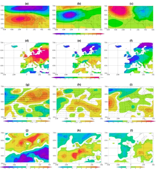
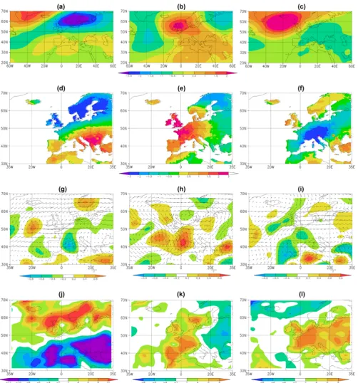
The second coupled mode again presents an EA-like pat-tern, despite some relevant differences in the dynamical fea-tures over Europe, such as the prevalence of low pressures over eastern Europe (Fig. 4b). As such, the EA is the sec-ond forcing on the occurrence of the wintertime tempera-ture extremes in Europe. Similar dynamical considerations to those already presented for the second coupling in the TN10p can be made here. The southwesterly flow over Europe leads to anomalously high occurrences of warm days over central and southeastern Europe (Fig. 4e), by inhibiting the northerly and easterly transports of cold air masses. The strong core of negative pressure located westwards of the British Isles also influences the temperatures throughout Scandinavia, where the number of occurrences of warm days is anomalously low (Fig. 4e). These conditions are also clearly favourable to the development of westerly transports over southwestern Europe (Fig. 4h) and to a resulting increase in cloudiness (Fig. 4k), which negatively feedbacks on the warm advec-tions and explains the relatively weak signal in the warm day occurrences over Iberia (Fig. 4e).
The third coupled mode reveals a West Atlantic (WA)-like pattern, also known by East Atlantic/western Russia pattern (Fig. 4c). This tri-pole pattern was identified by Wallace and Gutzler (1981) and was also referred to as the Eurasian pat-tern (type II) by Barnston and Livezey (1987). Two centres-of-action of the same signal are located near the Azores and over northeastern Europe, and a centre of opposite sig-nal is located over the high latitudes of the North Atlantic (Fig. 4c). In its positive phase (strong anticyclonic ridge over the high-latitude North Atlantic), below-normal occurrences of warm days over western Europe and northern Scandi-navia are shown (Fig. 4f). The strong northerly flows of arc-tic air masses over most of the continent (Fig. 4i) underlie these anomalously low temperatures and can often trigger prolonged cold spells. The southerly flows and their corre-sponding warm advections over the eastern Mediterranean (Fig. 4i) cause anomalously high occurrences of warm days. The enhanced (weakened) cloudiness over eastern (western) Europe partially offsets the temperature advections (Fig. 4l), decisively contributing to weakening the co-variability of this coupled mode. In the negative phase (strong trough over the high-latitude North Atlantic), the strong southerly flows of warm air masses over western and central Europe play a cen-tral role in settling warm weather conditions and in determin-ing above-normal occurrences of warm days over the western half of Europe (reversed patterns in Fig. 4c, f, i and l). 3.2 Summer extremes
3.2.1 Extreme value analysis
The assessment of extreme temperatures (TN10p and TX90p) in summer (JJA) is of utmost relevance for Europe, mainly due to the high vulnerability of many socio-economic sectors to their occurrence, particularly in the Mediterranean
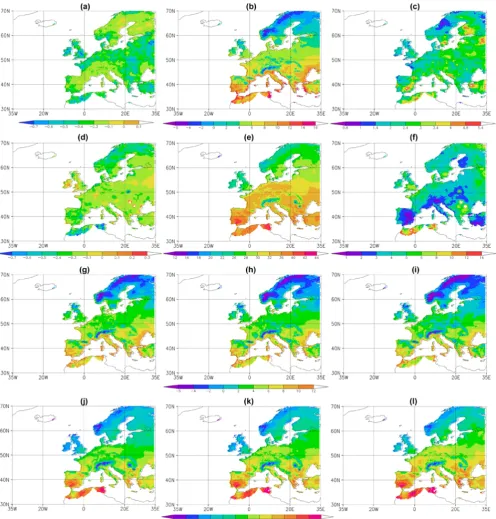
(e.g. Xoplaki et al., 2003; Jones et al., 2008). For instance, above-normal summer temperatures often trigger forest fires in the Mediterranean region, while below-normal values can also be harmful to crops, with detrimental implications in several socio-economic sectors. As for winter, GEV distri-butions were fitted to the summer TNN and TXX and their shape parameters suggest that the Gumbel family distribu-tions generally provide the best fits: negative or near-zero shape parameters (Fig. 5a and d). The mean fields are co-herent with the climate-mean patterns (Fig. 5b and e), while the variance fields exhibit relatively complex patterns, with-out a clear spatial coherence (Fig. 5c and f). The tempera-tures for the 5-, 10- and 20-yr return periods are also shown (Fig. 5g–l), again providing information, at a regional scale, of the exceptionality of a given temperature.
The monthly mean TN10p and TX90p fields (Fig. 6a–f) essentially reflect the climatological meridional temperature gradient and some orographic features, such as high-altitude regions. Statistically significant negative trends in TN10p can be observed throughout Europe, particularly over cen-tral Europe, France, the British Islands and Scandinavia and mainly in July and August (Fig. 6g–i). Conversely, upward trends are observed in TX90p throughout Europe (Fig. 6j– l). These trends revealed that cold nights (warm days) are becoming less (more) frequent in summer, as was already stated for winter (Luterbacher et al., 2004; Sch¨ar et al., 2004; Moberg and Jones, 2005; Alexander et al., 2006). These find-ings are also consistent with the results obtained by Kuglitsch et al. (2010) in their study of the heat waves in the eastern Mediterranean.
3.2.2 Large-scale coupling modes
As in the previous section, the BPCCA was also used to as-sess the relationships between the large-scale circulation and summer extreme temperature indices. For both indices only the most relevant modes were retained for the BPCCA (five PCs for TN10p and seven PCs for TX90p) that represent about 69 % and 71.4 % of the total variance, respectively, and five PCs for the MSLP representing 72.5 % of the total vari-ance. As for winter, only the first three coupled modes are considered here and their canonical correlations are approx-imately of 0.63, 0.52 and 0.39 for TN10p and of 0.69, 0.63 and 0.44 for TX90p.
prevents strong nighttime radiative cooling, it contributes to a decrease in the occurrence of cold nights and thereby to a strengthening of the negative anomalies over eastern Europe. The second coupled mode has a northerly displaced NAO-like pattern (a typical summertime regime) and can be con-nected to an intense North Atlantic ridge (Fig. 7b) that pro-duces a decrease in the occurrence of cold summer nights in the Iberian Peninsula, the British Isles and Scandinavia, whist in central Europe and in the Mediterranean, nights tend to be anomalously cold (Fig. 7e). The strong anticyclonic cir-culation over central Europe causes northerly flows and cold advections (Fig. 7h), settling dry weather conditions and low cloudiness over central Europe (Fig. 7k), which undoubt-edly favours cool nights (Fig. 7e). Moreover, the location and strength of the North Atlantic ridge favour the advec-tion of very warm air masses over western Iberia (Fig. 7h), thus being favourable to the establishment of warm episodes, or even heat waves, in the Iberian Peninsula and to below-normal occurrences of cold nights (Fig. 7e).
Lastly, the third coupled mode (Fig. 7c) can be associated with an Atlantic low regime (Cassou et al., 2005) that en-ables an overall reduction of the cold summer nights through-out Europe, with particular relevance over central Europe (Fig. 7f). The number of occurrences of warmer and drier nights in this area is linked to a southerly transport of warm air with its maximum strength over France (Fig. 7i). The role played by cloudiness is not very expressive in this mode and depends mostly on the region (Fig. 7l).
For the summer warm days (TX90p), the leading coupling between the MSLP and their frequency of occurrence has a pressure pattern with a dipolar structure over Europe with an important meridional pressure gradient over the continent (Fig. 8a). As a result, a north-south temperature contrast is induced, resulting in a reduction (increase) of warm summer days in northern (southern) Europe (Fig. 8d). This meridional contrast is clearly reflected in the cloud cover (Fig. 8j), which largely governs the forcing on the temperature. In fact, in the positive phase, the low-pressure systems over northern Eu-rope establish unstable weather conditions, with air parcel rising and cloud formation. Conversely, over southern Eu-rope, the high-pressure systems warrant atmospheric stabil-ity, subsidence and low cloudiness. In fact, for this mode, no clear association can be found with the temperature advec-tions, as they tend to be relatively weak (Fig. 8g). Conse-quently, on the contrary to the previous leading modes, this coupling appears to be mainly forced by cloudiness, rather than by advections, which are generally weak in a typical summertime atmospheric flow.
The second couple mode depicts a wave-like pattern with two negative cores (in the North Atlantic and Scandinavia) and a positive core over the British Isles (Fig. 8b). As a re-sult of this pattern, western Europe experiences an increase in the occurrences of summer warm days (Fig. 8e), mostly related to strong warm advections (Fig. 8h), despite the
en-hanced cloud cover (Fig. 8k). The third coupled mode dis-plays a Greenland anticyclone-like regime, with a strong core over Greenland and another, of opposite and weaker signal, extending from the North Atlantic towards Europe (Fig. 8c). This pattern also resembles the NAO-like summer pattern de-scribed by Hurrell et al. (2003), the blocking-like pattern by Liu (1994) and the blocking regime by Cassou et al. (2005). Overall, its large-scale conditions are related to high block-ing activity (Rimbu and Lohmann, 2011) that leads to an en-hancement of the easterlies over northern Europe. As a result, warm continental air is transported towards Scandinavia and the British Isles, whereas over the Iberian Peninsula and cen-tral Europe the advections of cold air result in a reduction in the number of summer warm days (Fig. 8f and i), which is enhanced by an increase in cloudiness (Fig. 8l). In the nega-tive phase, high pressure systems over Europe are accompa-nied by strong low pressure anomalies in the North Atlantic (reverse of Fig. 8c). The resulting southerly flows and warm advections over Europe (reverse of Fig. 8i), combined with low cloudiness (reverse of Fig. 8l), yield above-normal oc-currences of warm days (reverse of Fig. 8f). This atmospheric situation is indeed quite similar to that of the 2003 heat wave in Europe (Trigo et al., 2005; Della-Marta et al., 2007) and is an illustration of the potential this coupling may have to es-tablish extremely warm weather conditions across vast areas of Europe.
3.3 Transitional seasons: autumn and spring
3.3.1 Extreme value analysis
The spring monthly mean TN10p and TX90p fields (Fig. S3a–f) also reflect the climatological meridional tem-perature gradient and orographic features, as well as a clear month-to-month transition from winter to summer. This tran-sition is clearly depicted in the northern half of Europe, as temperatures will gradually increase to values close to those observed in summer. Despite being scattered, areas of sig-nificant negative trends in TN10p are found in March and April (Fig. S3g and h). In May, however, besides the nega-tive trends over western and central Europe, a wide area of significant positive trends can be found over eastern Europe (Fig. S3i). For the TX90p in spring months (Fig. S3j–l), sta-tistically significant negative trends are depicted over wide areas of Europe, in opposition to the upward trends observed in the summer months (Fig. 6j–l).
Both TN10p and TX90p monthly mean fields in the au-tumn months (Fig. S4a–f) reveal minimum values over north-ern and eastnorth-ern Europe and higher values over southnorth-ern and western Europe. However, it is worth mentioning the sharp transition from September to November in both indices. The number of cold days in the north becomes higher and un-dergoes a southward displacement, whereas the number of warm days (similar to the ones observed in summer Fig. 2d– f), mainly in September, decreases and becomes more con-fined to the Iberian Peninsula. No spatially coherent statisti-cally significant trends are found for September and Novem-ber TN10p (Fig. S4g and i). Nevertheless, significant posi-tive trends are observed in October, particularly over Scan-dinavia and eastern Europe (Fig. S4h). Although less signif-icant than the trends observed during the TX90p in summer months (Fig. 6j–l), several significant positive trends are also depicted for TX90p (Fig. S4j–l): namely, over large areas of eastern Europe in September and November, over the Iberian Peninsula and northern Europe in October. The TX90p in au-tumn months shows significant positive trends (more warm days), mainly over eastern Europe. Hence, the previous out-comes show that in spring (autumn) there is a trend for a decrease (increase) in the number of both temperature ex-tremes. These findings are also in agreement with previous studies (e.g. Xoplaki et al., 2005).
3.3.2 Large-scale coupling modes
For spring, the most relevant modes were retained for BPCCA (4 PCs for TN10p and 6 PCs for TX90p) that repre-sent about 72.5 % and 72.7 % of the total variance, respec-tively, and 3 PCs for the MSLP, representing 71 % of the total variance. Only the leading coupled mode is statisti-cally significant and has a canonical correlation of 0.39 for TN10p and 0.47 for TX90p. Following the same methodol-ogy for autumn, 5 PCs for TN10p, 6 PCs for TX90p (69.2 % and 70.1 % of the total variance, respectively) and 4 PCs for the MSLP (69.7 % of the total variance) were retained for BPCCA. Again, only the first coupled mode is significant,
with a canonical correlation of 0.36 for TN10p and 0.34 for TX90p.
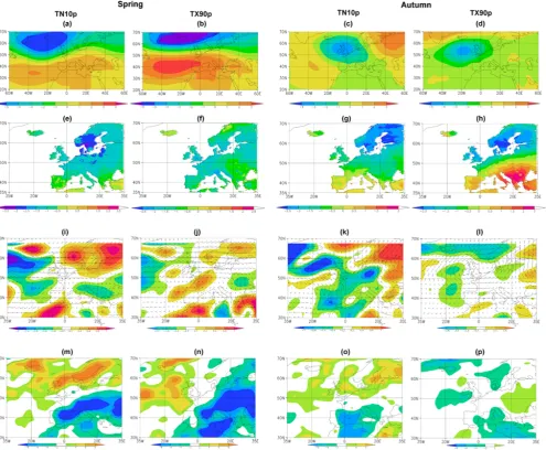
The large-scale couplings for the transitional seasons (spring and autumn) are now inspected. As there are im-portant similarities with the previously presented modes for winter and for summer, their dynamical characterization is only shortly referred here. In spring, the leading coupled modes for both TN10p and TX90p reveal high similarity with the corresponding leading winter modes (Figs. 3, 4 and 9a and b), being in both cases a manifestation of the NAO. In fact, despite some differences in detail, the anomalies in the large-scale atmospheric circulation are highly compara-ble (Figs. 3a, 4a and 9a and b). Furthermore, the forcing of each coupled mode on the frequencies of occurrence of extremes, on temperature advections and on cloudiness, is largely coherent with the previous large-scale patterns and resembles the respective winter patterns (Figs. 3, 4 and 9). Therefore, the previous dynamical considerations for winter can be easily extended to the spring modes and will not thus be repeated here. For the autumn, however, the leading pat-terns show EA-like structures for both indices (Fig. 9c and d). The presence of low pressure systems over the British Isles is associated with anomalously low (high) occurrences of cold nights in northern (southern) Europe. On the other hand, the presence of low pressure systems westwards of the British Isles is associated with anomalously low (high) oc-currences of warm days in northern (southern) Europe. These couplings can also be largely connected to temperature ad-vections (Fig. 9k and l) and cloudiness (Fig. 9o and p).
4 Summary and conclusions
Fig. 9. Leading coupled mode for the spring (MAM) for (a, e) MSLP (in hPa SD−1)and TN10p index (in days month−1SD−1), and for (b, f) MSLP (in hPa SD−1)and TX90p index (in days month−1SD−1)in 1961–2010. Canonical correlations are respectively 0.39 and 0.47 (95 % confidence level). Differences between the positive and negative phases of the spring coupled mode for the temperature advection (shaded in K s−1)and horizontal wind (arrows in m s−1)at 850 hPa (i) TN10p index (j) TX90p index and for the total cloud cover (in %) (m) TN10p index and (n) TX90p index in 1961–2010. Panels (c, d, g, h) the same as for (a, b, e, f) but for the autumn (SON) leading coupled mode. Canonical correlations are respectively 0.36 and 0.34 (95 % confidence level). Panels (k, l, o, p) the same as (i, j, m, n) but for the differences between the positive and negative phases of the autumn coupled mode.
the TN10p (TX90p) in spring months, statistically signifi-cant negative trends (less extremes) are depicted over scat-tered (wide) areas of Europe (Fig. S3g–l). In autumn, signifi-cant positive trends (more extremes) were found in northeast-ern Europe for the TX90p (Fig. S4j–l), whilst for the TN10p spatially coherent significant trends were found in October (more cold nights in northeastern Europe; Fig. S4k). These findings are in contrast with the increase in warm days and slight changes in cold days detected for winter and summer.
The large-scale atmospheric forcing on the variability of the TN10p and TX90p is here discussed by applying the
1992; Hurrell and van Loon, 1997; Jones et al., 1997). This forcing is particularly evident not only in the mean air tem-peratures over central and northern Europe (e.g. Xoplaki et al., 2003; Luterbacher et al., 2004; Della-Marta et al., 2007), but also on their extremes (e.g. Santos and Corte-Real, 2006). The second wintertime coupling in both TN10p and TX90p is mainly a manifestation of the influence of the EA on the temperature extremes in Europe, despite some impor-tant differences in the pattern associated with each extreme (Figs. 3b and 4b). On the whole, in its positive phase, this coupled mode triggers important warm advections over Eu-rope, driven by southwesterly flows. These warm advections prevent the occurrence of extremely cold nights over most of western and central Europe (Fig. 3e and h), being also reinforced by the enhanced cloudiness (low outgoing long-wave fluxes and less radiative cooling) over southwestern Europe (Fig. 3k). Conversely, these warm advections favour the occurrence of exceptionally warm days over several re-gions of western, central and southeastern Europe (Fig. 4e and h), though the enhanced cloudiness (low incoming short-wave fluxes and less radiative warming) partially offsets the warm advection effects over southwestern Europe (Fig. 4k). In spite of some noteworthy differences between both in-dices, the third coupling essentially reveals a phase opposi-tion between the MSLP over Europe and the high-latitudes of the North Atlantic and Greenland (Figs. 3c and 4c). In its positive phase (strong high pressure systems northwestwards of Europe), it does not prevent the occurrence of cold out-breaks over northern Europe (Fig. 3f), while its cold advec-tions driven by northerly winds (Fig. 4i) impede the occur-rence of warm days over most of Europe, particularly over Scandinavia and western Europe (Fig. 4f). The summer cou-plings are less coherent between both extreme indices. For the TN10p, the first coupling displays a wave-like pattern with three centres-of-action (Fig. 7a). In its positive phase, a strengthened North Atlantic ridge accompanied by low pres-sure systems over the Brinish Isles and the North Sea gener-ate cold advections by northerly transports of maritime cold air masses over western Europe (Fig. 7g), leading to above-normal occurrences of cold nights, particularly over south-western Europe (Fig. 7d). On the other hand, high pressure systems over northeastern Europe drive southerly winds and warm advections over eastern Europe (Fig. 7g), explaining the below-normal occurrences of cold-nights (Fig. 7d). En-hanced cloudiness over eastern Europe also helps strength-ening this signal (Fig. 7j). The second order coupling in sum-mer TN10p shows a northeastwardly displaced Azores high, with a ridge over central Europe and an inverted trough over northwest Africa and Portugal (Fig. 7b). Cold advections and low cloudiness (Fig. 7h and k) explain above-normal occur-rences of cold nights over large areas of southern and cen-tral Europe (Fig. 7e). Westerly winds over northern Scandi-navia and warm advections by southeasterly winds over the southwestern Iberian Peninsula explain the opposite signal in the occurrence of cold nights (Fig. 7e). Lastly, the third
coupled mode presents a dipolar structure (Fig. 7c). In its positive phase, low pressure systems over the North Atlantic and high pressure systems over northeastern Europe induce warm advections over almost all of Europe (Fig. 7i) that lead to below-normal occurrences of cold nights (Fig. 7f). Low (high) cloudiness over northeastern (southeastern) Eu-rope also plays a role in this forcing (Fig. 7l).
The summer forcing on TX90p shows that the meridional pressure gradient over Europe plays a key role in the oc-currence of warm days over the continent (Fig. 8a). When low pressure systems occur over northern Europe and are ac-companied by relatively high pressures over southern Europe (positive phase), below-normal (above-normal) occurrences of warm days are verified over northern (southern) Europe (Fig. 8a and d). The temperature advections are not a ma-jor forcing factor for this mode (Fig. 8g). Nevertheless, high (low) cloudiness over northern (southern) Europe is clearly related to the low (high) occurrence of extremely high warm days (Fig. 8j), since it strongly controls the daytime solar radiative fluxes on the surface. Exceptionally warm sum-mer days over western Europe (Fig. 8e) can be associated with a blocking high pressure system centred over the British Isles (Fig. 8b) that induces warm advections over the region (Fig. 8h) and low cloudiness (Fig. 8k). Summer warm days over large areas of Europe (Fig. 8f), particularly over cen-tral Europe, can also be triggered by high pressure systems over the continent that block the westward progression of the North Atlantic low pressure systems (Fig. 8c). These condi-tions lead to warm adveccondi-tions and to low cloudiness over the continent (Fig. 8i and l) that jointly contribute to the occur-rence of exceptionally warm episodes. The analysis of the transitional seasons (spring and autumn) revealed that the NAO is the leading coupling in spring and for both indices (Fig. 9a and b), whereas EA-like oscillations are the leading patterns in autumn and also for both indices (Fig. 9c and d).
The results obtained in the present study help clarifying the main large-scale forcing mechanisms on the occurrence of temperature extremes in Europe and are consistent with the statistical behaviour of the TNN and TXX (Figs. 1, 5, S1 and S2). Although previous studies have already been devoted to this subject, in the present study, the role that large-scale atmospheric circulation plays in the temperature extremes in Europe is further explored by applying alter-native approaches and by considering an updated (1961– 2010) state-of-the-art observational dataset (E-OBS), with gridded data defined at a comparably high spatial resolu-tion (0.25◦latitude×0.25◦longitude). The outcomes of this
other potentially important factors, such as local effects on weather, caused by orography, water bodies and breezes, among other microclimate features. These features would in-deed require higher resolution datasets and more regionally focused studies. The main statistical methodology used here (BPCCA) is also unsuitable for the local-scale analysis, as it is precisely developed to isolate dominant large-scale co-variability patterns, filtering out small-scale details. In a fu-ture work it is projected to test the skill of global circulation models in reproducing the coupled modes and to produce, af-ter an adequate model validation/calibration, climate change projections for these modes.
Supplementary material related to this article is available online at:
http://www.nat-hazards-earth-syst-sci.net/12/1671/2012/ nhess-12-1671-2012-supplement.zip.
Acknowledgements. We acknowledge the E-OBS dataset from EU-FP6 project ENSEMBLES (http://ensembles-eu.metoffice.com) and the data providers in the ECA&D project (http://eca.knmi.nl). This work was supported by European Union Funds (FEDER/COMPETE – Operational Competitiveness Programme) and by national funds (FCT – Portuguese Foundation for Science and Technology) under the project FCOMP-01-0124-FEDER-022696. All maps were produced by the Grid Analysis and Display System developed for Ocean-Land-Atmosphere Interactions. The authors are grateful to the two excellent reviewers who significantly contributed to improve the paper.
Edited by: R. Trigo
Reviewed by: two anonymous referees
References
Alexander, L. V., Zhang, X., Peterson, T. C., Caesar, J., Glea-son, B., Tank, A. M. G., Haylock, M., Collins, D., Trewin, B., Rahimzadeh, F., Tagipour, A., Ambenje, P., Kumar, K., Re-vadekar, J., and Griffiths G.: Global observed changes in daily climate extremes of temperature and precipitation, J. Geophys. Res., 111, D05109, doi:10.1029/2005JD006290, 2006.
Andrade, C., Santos, J. A., Pinto, J. G., and Corte-Real, J.: Large-scale atmospheric dynamics of the wet winter 2009-2010 and its impact on hydrology in Portugal, Clim. Res., 46, 29–41, doi:10.3354/cr00945, 2011.
Barnett, T. P. and Preinsendorfer, R.: Origins and levels of monthly and seasonal forecast skill for United States surface air tem-peratures determined by canonical correlation analysis, Mon. Weather Rev., 115, 1825–1850, 1987.
Barnston, A. G. and Livezey, R. E.: Classification, seasonality and persistence of low-frequency atmospheric circulation patterns, Mon. Weather Rev., 115, 1083–1126, 1987.
Bretherton, C. S., Smith, C., and Wallace, J. M.: An intercompar-ison of methods for finding coupled patterns in climate data, J. Climate, 5, 541–560, 1992.
Bueh, C. and Nakamura, H.: Scandinavian pattern and its cli-matic impact, Q. J. R. Meteorol. Soc., 133, 2117–2131, doi:10.1002/qi.173, 2007.
Carril, A. F., Gualdi, S., Cherchi, A., and Navarra, A.: Heatwaves in Europe: Areas of homogenous variability and links with the regional to large-scale atmospheric and SSTs anomalies, Clim. Dynam., 30, 77–98, 2008.
Cassou, C., Terray, L., and Phillips, A. S.: Tropical Atlantic Influ-ence on European Heat Waves, J. Climate, 18, 2805–2811, 2005. Casty, C., Wanner, H., Luterbacher, J., Esper, J., and B¨ohm, R.: Temperature and precipitation variability in the European Alps since 1500, Int. J. Climatol., 25, 1855–1880, 2005.
Chase, T. N., Wolter, K., Pielke Sr., R. A., and Rasool, I.: Was the 2003 European summer heat wave unusual in a global context?, Geophys. Res. Lett., 33, L23709, doi:10.1029/2006GL027470, 2006.
Coles, S.: An Introduction to Statistical Modeling of Extreme Val-ues, Springer, 208 pp., 2001.
Corte-Real, J., Zhang, Z., and Wang, X.: Large-scale circulation regimes and surface climatic anomalies over the Mediterranean, Int. J. Climatol., 15, 1135–1150, 1995.
Costa, A. C., Santos, J. A., and Pinto, J. G.: Climate change scenar-ios for precipitation extremes in Portugal, Theor. Appl. Climatol., 108, 217–234, doi:10.1007/s00704-011-0528-3, 2012.
Della-Marta, P. M., Haylock, M. R., Luterbacher, J., and Wanner, H.: Doubled length of western European summer heat waves since 1880, J. Geophys. Res., 112, D15103, doi:10.1029/2007JD008510, 2007.
Diffenbaugh, N. S., Pal, J. S., Giorgi, F., and Gao, X.: Heat stress in-tensification in the Mediterranean climate change hotspot, Geo-phys. Res. Lett., 34, L11706, doi:10.1029/2007GL030000, 2007. Easterling, D. R., Meehl, G. A., Parmesan, C., Changnon, S. A., Karl, T. R., and Mearns, L. O.: Climate extremes: observations, modeling, and impacts, Science, 289, 2068–2074, 2000. Ferris, R., Ellis, R. H., Wheeler, T. R., and Hadley, P.: Effect of
high temperature stress at anthesis on grain yield and biomass of field-grown crops of wheat, Ann. Bot., 82, 631–639, 1998. Folland, C. K., Miller, C., Bader, D., Crowe, M., Jones, P.,
Plum-mer, N., Richman, M., Parker, D. E., Rogers, J., Scholefield, P., and Lee, J. Q.: Workshop on indices and indicators for climate extremes, Asheville, NC, USA, 3–6 June 1997-Breakout group C: temperature indices for climate extremes, Climatic Change, 42, 31–43, 1999.
F¨orster, H. and Lilliestam, J.: Modelling Thermoelectric Power Generation in View of Climate Change, Reg. Environ. Change, 11, 211–212, 2010.
Giorgi, F.: Climate change hot-spots, Geophys. Res. Lett., 33, L08707, doi:10.1029/2006GL025734, 2006.
Guirguis, K., Gershunov, A., Schwartz, R., and Bennett, S.: Re-cent warm and cold daily winter temperature extremes in the Northern Hemisphere, Geophys. Res. Lett., 38, L17701, doi:10.1029/2011GL048762, 2011.
Haylock, M. R., Hofstra, N., Klein Tank, A. M. G., Klok, E. J., Jones, P. D., and New, M.: A European daily high-resolution gridded dataset of surface temperature and precipitation, J. Geo-phys. Res. Atmos., 113, D20119, doi:10.1029/2008JD10201, 2008.
Hurrell, J. W.: Decadal trends in the North Atlantic Oscillation: Re-gional temperatures and precipitation, Science, 269, 676–679, 1995.
Hurrell, J. W. and van Loon, H.: Decadal variations in climate asso-ciated with the North Atlantic Oscillation, Climatic Change, 36, 301–326, 1997.
Hurrell, J. W., Kushnir, Y., Ottersen, G., and Visbeck, M.: An overview of the North Atlantic Oscillation. The North Atlantic Simulation: Climate Significance and Environmental Impacts, Geophys. Monogr., No. 134, 1–22, 2003.
IPCC: (International Panel on Climate Change), Climate Change 2007, Impacts, Adaptation and Vulnerability, Cambridge, Cam-bridge University Press, 2008.
Jenkinson, A. F.: The frequency distribution of the annual maximum (or minimum) values of meteorological elements, Q. J. Roy. Me-teorol. Soc., 81, 158–171, 1955.
Jones, G. S., Stott, P. A., and Christidis, N.: Human contri-bution to rapidly increasing frequency of very warm North-ern Hemisphere summers, J. Geophys. Res., 113, D02109, doi:10.1029/2007JD008914, 2008.
Jones, P. D., Osborn, T. J., and Briffa, K. R.: Estimating sampling errors in large-scale temperature averages, J. Climate, 10, 2548– 2568, 1997.
Jones, P. D., Horton, E. B., Folland, C. K., Hulme, M., Parker, D. E., and Basnett, T. A.: The use of indices to identify changes in climatic extremes, Climatic Change, 42, 131–149, 1999. Kalnay, E., Kanamitsu, M., Kistler, R., Collins, W., Deaven, D.,
Gandin, L., Iredell, M., Saha, S., White, G., Woollen, J., Zhu, Y., Leetmaa, A., Reynolds, R., Chelliah, M., Ebisuzaki, W., Higgins, W., Janowiak, J., Mo, K. C., Ropelewski, C., Wang, J., Jenne, R., and Joseph, D.: The NCEP/NCAR 40-year reanalysis project, B. Am. Meteorol. Soc., 77, 437–470, 1996.
Karl, T. R., Nicholls, N., and Ghazi, A.: CLIVAR/GCOS/WMO workshop on indices and indicators for climate extremes: Work-shop summary, Climatic Change, 42, 3–7, 1999.
Koch, H. and V¨ogele, S.: Dynamic Modeling of Water Demand, Water Availability and Adaptation Strategies for Power Plants to Global Change, Ecol. Econ., 68, 2031–2039, 2009.
Kuglitsch, F. G., Toreti, A., Xoplaki, E., Della-Marta, P. M., Zere-fos, C. S., T¨urkes, M., and Luterbacher, J.: Heat wave changes in the eastern Mediterranean since 1960, Geophys. Res. Lett., 37, L04802, doi:10.1029/2009GL041841, 2010.
Liu, Q.: On the definition and persistence of blocking, Tellus, 46A, 286–298, 1994.
Luterbacher, J., Dietrich, D., Xoplaki, E., Grosjean, M., and Wan-ner, H.: European seasonal and annual temperature variability, trends, and extremes since 1500, Science, 303, 1499–1503, 2004. Milligan, J.: Heatwaves: the developed world’s hidden disaster, Techn. Ber., International Federation of Red Cross and Red Cres-cent, World Disasters Report, 2004.
Moberg, A. and Jones, P. D.: Trends in indices for extremes in daily temperature and precipitation in central and western Eu-rope, 1901–99, Int. J. Climatol., 25, 1149–1171, 2005.
Moriondo, M., Good, P., Dur˜ao, R., Bindi, M., Giannakopou-los, C., and Corte-Real, J.: Potential impact of climate change on fire risk in the Mediterranean area, Clim. Res., 31, 85–95, doi:10.3354/cr031085, 2006.
Pereira, M. G., Trigo, R., da Camara, C., Pereira, J., and Leite, S. M.: Synoptic patterns associated with large summer
forest fires in Portugal, Agr. Forest Meteorol., 129, 11-25, doi:10.1016/j.agrformet.2004.12.007, 2005.
Peterson, T. C.: Climate Change Indices, WMO Bulletin, 54, 83–86, 2005.
Pinto, J. G. and Raible, C. C.: Past and recent changes in the North Atlantic oscillation, WIREs, Climatic Change, 3, 79–90, doi:10.1002/wcc.150, 2012.
Poumad`ere, M., Mays, C., Le Mer, S., and Blong, R.: The 2003 heat wave in France: dangerous climate change here and now, Risk. Anal., 25, 1483–1494, 2005.
Pozo-V´azquez, D., Esteban-Parra, M. J., Rodrigo, F. S., and Castro-D´ıez, Y.: A study of NAO variability and its possible non-linear influences on European surface temperature, Clim. Dynam., 17, 701–715, 2001.
Rimbu, N. and Lohmann, G.: Winter and summer blocking variabil-ity in the North Atlantic region – evidence from long-term ob-servational and proxy data from southwestern Greenland, Clim. Past, 7, 543–555, doi:10.5194/cp-7-543-2011, 2011.
Robine, J., Cheung, S., Le Roy, S., Van Oyen, H., Griffiths, C., Michel, J., and Herrmann, F.: Death toll exceeded 70,000 in Eu-rope during the summer of 2003, Comptes Rendus Biologies, 331, 171–178, doi:10.1016/j.crvi.2007.12.001, 2008.
Rodr´ıguez-Puebla, C., Encinas, A. H., Garc´ıa-Casado, L. A., and Nieto, S.: Trends in warm days and cold nights over the Iberian Peninsula: relationships to large-scale variables, Climatic Change, 100, 667–684, doi:10.1007/s10584-009-9721-0, 2010. Santos, J. and Corte-Real, J.: Temperature Extremes in Europe and
Large-Scale Circulation: HadCM3 future scenarios, Clim. Res., 31, 3–18, 2006.
Santos, J., Corte-Real, J., and Leite, S.: Atmospheric large-scale dy-namics during the 2004–2005 winter drought in Portugal, Int. J. Climatol., 27, 571–586, 2007.
Santos, J. A., Andrade, C., Corte-Real, J., and Leite, S.: The role of large-scale eddies in the occurrence of precipitation deficits in Portugal, Int. J. Climatol., 29, 1493–1507, doi:10.1002/joc.1818, 2008.
Scaife, A. A., Folland, C. K., Alexander, L. V., Moberg, A., and Knight, J. R.: European climate extremes and the North Atlantic Oscillation, J. Climate, 21, 72–83, 2008.
Sch¨ar, C., Vidale, P. L., Luthi, D., Frei, C., Haberli, C., Liniger, M. A., and Appenzeller, C.: The role of increasing temperature variability in European summer heatwaves, Nature, 427, 332– 336, 2004.
Trigo, R. M., Osborn, T. J., and Corte-Real, J.: The North Atlantic Oscillation influence on Europe: climate impacts and associated physical mechanisms, Clim. Res., 20, 9–17, 2002.
Trigo, R. M., Garc´ıa-Herrera, R., D´ıaz, J., Trigo, I. F., and Valente, M. A.: How exceptional was the early August 2003 heatwave in France?, Geophys. Res. Lett., 32, L10701, doi:10.1029/2005GL022410, 2005.
von Storch, H. and Zwiers, F. M.: Statistical analysis in climate re-search, Cambridge University Press, Cambridge, 1999. Wallace, J. M. and Gutzler, D. S.: Teleconnection in the
geopoten-tial height field during the Northern Hemisphere winter, Mon. Weather Rev., 109, 784–812, 1981.
WHO: The health impacts of 2003 summer heat-waves, Briefing note for the Delegations of the fifty-third session of the WHO (World Health Organization) Regional Committee for Europe, 12 pp., 2003.
Wilks, D. S.: Statistical methods in the atmospheric sciences, Aca-demic Press, USA, 2006.
Xoplaki, E., Gonzalez-Rouco, J., Luterbacher, J., and Wanner, H.: Mediterranean summer air temperature variability and its con-nection to the large-scale atmospheric circulation and SSTs, Clim. Dynam., 20, 723–739, 2003.
Xoplaki, E., Luterbacher, J., Paeth, H., Diertrich, D., Steiner, N., Grosjean, M., and Wanner, H.: European spring and au-tumn temperature variability and change of extremes over the last half millennium, Geophys. Res. Lett., 32, L15713, doi:10.1029/2005GL023424, 2005.