www.nat-hazards-earth-syst-sci.net/10/171/2010/ © Author(s) 2010. This work is distributed under the Creative Commons Attribution 3.0 License.
Natural Hazards
and Earth
System Sciences
On analysing sea level rise in the German Bight since 1844
T. Wahl, J. Jensen, and T. Frank
Research Institute for Water and Environment, University of Siegen, Germany
Received: 27 July 2009 – Revised: 4 January 2010 – Accepted: 17 January 2010 – Published: 1 February 2010
Abstract. In this paper, a methodology to analyse observed
sea level rise (SLR) in the German Bight, the shallow south-eastern part of the North Sea, is presented. The paper fo-cuses on the description of the methods used to generate and analyse mean sea level (MSL) time series. Parametric fitting approaches as well as non-parametric data adaptive filters, such as Singular System Analysis (SSA) are applied. For padding non-stationary sea level time series, an advanced ap-proach named Monte-Carlo autoregressive padding (MCAP) is introduced. This approach allows the specification of un-certainties of the behaviour of smoothed time series near the boundaries. As an example, the paper includes the results from analysing the sea level records of the Cuxhaven tide gauge and the Heligoland tide gauge, both located in the south-eastern North Sea. For comparison, the results from analysing a worldwide sea level reconstruction are also pre-sented. The results for the North Sea point to a weak negative acceleration of SLR since 1844 with a strong positive accel-eration at the end of the 19th century, to a period of almost no SLR around the 1970s with subsequent positive acceleration and to high recent rates.
1 Introduction
Sea Level Rise (SLR) is one of the major consequences we are facing in times of a warming climate and it is obvious that a higher sea level influences the heights of occurring storm surges and thus results in a higher risk of inundation for the affected coastal areas. Therefore, regional and global sea level rise are subjects to many recent scientific publications (e.g., White et al., 2005; Jevrejeva et al., 2006; W¨oppelmann et al., 2006; Holgate, 2007; Church et al., 2008; Woodworth
Correspondence to: T. Wahl ([email protected])
et al., 2009a, b). In contrast, the mean sea level (MSL) and its variability over the last centuries in the German North Sea area have not been analysed in detail up to now. This is sur-prising, because many long and continuous sea level time series are available (Wahl et al., 2008). Some studies consid-ered time series from a very small number of tide gauges and high resolution data sets have not been used or not been available (e.g. Dietrich, 1954; Jensen and Mudersbach, 2007). Furthermore, various projects dealing with mean tidal conditions, e.g. the mean tidal high waters (MHW) or the mean tidal ranges (MTR), have been conducted so far (e.g., F¨uhrb¨oter and Jensen, 1985; T¨oppe and Brockmann, 1992; G¨onnert et al., 2004). Most of the available sea level records consist of high and low water heights and times (from here on referred to as high and low waters), which are not directly applicable for MSL analyses. The simple averaging of high and low waters leads to the mean tide level (MTL) and not to the MSL. The latter can be estimated by averaging high resolution sea level data consisting of at least hourly mea-surements. The difference between MSL and MTL is small in most areas (e.g., Pugh, 2004; W¨oppelmann et al., 2006), but up to more than 20 cm along the German North Sea coast-line due to shallow water effects (Lassen, 1989). This has to be considered when generating and analysing mean sea level time series. In addition, some differences between observa-tions and model results, often referred to as “negative sea level budget” (e.g., Church et al., 2008), have not been com-pletely understood up to now. All the more important is the proper analysis of available data sets from tide gauges and in the recent past also from satellites.
The present paper has three main objectives. The first one is to introduce a method which is easy to apply to combine MSL and MTL data. The second one is to introduce an ad-vanced method for padding or extrapolating time series be-fore applying any smoothing technique to find the optimal fit. The third one is to analyse sea level records from two tide gauges in the German North Sea.
172 T. Wahl et al.: On analysing sea level rise in the German Bight since 1844 To address the first objective, a modification of the so
called k-factor method is introduced in Sect. 2 (Lassen, 1989; Lentz, 1879; Wahl et al., 2008). This modification allows the consideration of non-stationarities in k-factor time series, where the k-factor is subsequently used to convert MTL to MSL. Based upon the resulting MSL time series, long-term trend estimations are possible and smoothing techniques can be applied without leading to gaps. The latter usually occurs, if time series consisting of MSL and MTL data are analysed without applying any methods to combine both variables. In addition, a shift of up to more than 20 cm somewhere in the time series certainly leads to significant errors and misinter-pretations when performing long-term trend estimations. It is worth noting that sea level time series from the German North Sea area show high variability because the major part of the sea level is influenced by stochastic meteorological processes (M¨uller-Navarra and Giese, 1999). Therefore, it is not always possible to detect shifts of ten to twenty centime-tres just by looking at the time series.
As mentioned above, the second objective of the paper is to introduce an advanced method for padding time series be-fore applying any smoothing technique. Whenever smooth-ing a time series, one has two opportunities. The first one is to start and stop the smoothing at a specified time (depend-ing on the chosen window length) before reach(depend-ing the ends of the original time series. For example a moving average with a window length of 19 years usually starts 9 years later than the original time series and ends 9 years earlier. The second op-portunity, which is increasingly applied in combination with the analysis of climate time series, is to find some meaning-ful extrapolation from a physical point of view, before ap-plying any smoothing technique. This enables the smoothed time series to cover the same period as the original time se-ries. The method presented in this paper, namely Monte-Carlo autoregressive padding (MCAP), results in a very data adaptive smooth and allows the specification of uncertainties near the boundaries due to the padding. Especially the latter is not the case with any other common techniques (e.g., Ghil et al., 2002; Mann, 2004; Jevrejeva et al., 2006; Jansen et al., 2007; Trenberth et al., 2007; Mann, 2008). But, to under-stand recent SLR and to find projections for the near future, especially the behaviour of the time series near the posterior boundary is important.
The third objective is addressed by presenting the results from analysing sea level records from two important tide gauges in the German North Sea. The Cuxhaven tide gauge provides the longest record with data since 1844. The He-ligoland tide gauge provides high quality data due to its ex-posed location (see Sect. 2). In a further step, the results from analysing the North Sea sea level time series are compared to global patterns of SLR derived from analysing a global sea level reconstruction. The results contribute to the verifica-tion of regional climate models and provide indicaverifica-tions of SLR for regional and local planning issues. This seems to be of special importance. First, the most recent SLR
sce-narios published by the Intergovernmental Panel on Climate Change (IPCC) (Meehl et al., 2007) are subject to an exten-sive scientific discussion. Some authors find hints from ob-servations or semi-empirical models that the scenarios might underestimate future SLR (Rahmstorf, 2007; Rahmstorf et al., 2007; Jevrejeva et al., 2008; Grinsted et al., 2009). It has to be noted, that the results from semi-empirical models, us-ing empirical relationships between temperature and SLR to estimate future projections, are also lively discussed by the scientific community (e.g. Holgate et al., 2007; von Storch et al., 2008). Second, and even more important, it has to be tested whether a significant correlation exists between SLR in the German North Sea region and global SLR.
2 Data and methods
Figure 1 shows the location of the Cuxhaven tide gauge and the Heligoland tide gauge in the south-eastern North Sea. The Cuxhaven station is located at the Elbe estuary and pro-vides permanent sea level data from 1844 to 2008. From the beginning of the record until 1918 only high and low waters are available and afterwards high resolution data with at least hourly values. The Heligoland station is installed in the har-bour of the island of Heligoland (Rohde, 1990), which is lo-cated about 62 kilometres north-westerly of the Elbe Estuary. Due to its exposed location in the deep water, the tide gauge provides almost unaffected sea level measurements and the tide curves are less deformed. High resolution data is pro-vided since 1953, with a period from 1990 to 1999 where only high and low waters are available.
Both data sets were corrected for local datum shifts and for glacial isostatic adjustment (GIA) by considering a rate of land subsidence of 0.34 mm a−1for the Cuxhaven sea level
time series and of 0.51 mm a−1for the Heligoland sea level time series (Peltier, 2004). GIA is a global process in re-sponse to large scale changes in the surface mass load result-ing from the last deglaciation. The effect of GIA (rebound or subsidence) is usually assumed to be linear, at least over the last couple of hundred years. Other geological effects may also contribute to land subsidence or rebound (e.g. tec-tonics, volcanic activity, withdraw of natural resources etc.), but GIA is the only one assessable through numerical mod-els. The sum of all the other effects can be measured via GPS, whereas the GPS station should be located near the tide gauge. Such measurements will contribute to the uncertainty reduction in further studies (Sch¨one et al., 2009) (see also Sect. 4).
T. Wahl et al.: On analysing sea level rise in the German Bight since 1844 173
17
Figures
491
492
4o
W 0o 4oE 8oE 12oE
48o
N
52o
N
54o
N
56o
N
58o
N
60o
N
50o
N
493
Fig. 1.
Locations of the tide gauges Cuxhaven and Heligoland in the south-eastern North Sea.
494
495
-100 0 100
S
L
R [
mm]
-100 0 100
1850 1900 1950 2000 2050 -100
0 100
Time [a]
SLR
[
m
m]
1850 1900 1950 2000 2050 0
200 400
Time [a] Observation AR1 model result
(a)
(c)
(b)
(d)
496
Fig. 2.
Steps of MCAP: (a) detrended annual Cuxhaven MSL time series, (b) result of the
497
AR1 Model, two times the chosen embedding dimension longer than the observed time series,
498
(c) padded detrended annual Cuxhaven MSL time series, using the ends of the result of the
499
AR1 model, (d) padded annual Cuxhaven MSL time series with long term-trend of the
500
observed time series re-included. Steps (b) to (d) are repeated 10,000 times through Monte
501
Carlo Simulations.
502
503
Fig. 1. Locations of the tide gauges Cuxhaven and Heligoland in the south-eastern North Sea.
the time period providing high resolution data using Eq. (1) (Lassen, 1989):
k(t )=(MHW(t )−MSL(t ))
MTR(t ) , (1)
where MHW(t) is the monthly mean high water, MSL(t) is the monthly mean sea level and MTR(t) is the monthly mean tidal range. For the German North Sea coastline, k-factors are found to vary between 0.43 and 0.49. A k-factor of 0.5 means that the tide curve has a perfect sinusoidal form and that MSL equals MTL.
Before combining MSL and MTL time series, it has to be tested whether the k-factor is a stationary parameter for the investigated gauge station or whether it shows non-stationary behaviour. Therefore, two tests on stationarity are applied to the monthly k-factor time series. The first one is a sliding-window test with a sliding-window length of one year to account for possible seasonality (Mudersbach and Jensen, 2008; van Gelder, 2008). The second test is a two-dimensional non-parametric Kolmogorov-Smirnov test (Chen and Rao, 2002; Mudersbach and Jensen, 2008). If the k-factor is found to be stationary, a monthly MSL time series can be easily esti-mated with Eq. (2):
MSL(t )=MTR(t )·(0.5−k)+MTL(t ), (2) where MSL(t) is the monthly mean sea level, MTR(t) is the monthly mean tidal range, k is the mean k-factor esti-mated from the time period providing high resolution data and MTL(t) is the monthly mean tide level. If the k-factor shows non-stationary behaviour, a first or higher order poly-nomial fit has to be applied and extrapolated before
correct-17
Figures
491
492
4o
W 0o
4oE 8oE 12 oE
48o
N
52o
N
54o
N
56o
N
58o
N
60o
N
50o
N
493
Fig. 1.
Locations of the tide gauges Cuxhaven and Heligoland in the south-eastern North Sea.
494
495
-100 0 100
S
L
R [
mm]
-100 0 100
1850 1900 1950 2000 2050 -100
0 100
Time [a]
SLR
[
m
m]
1850 1900 1950 2000 2050 0
200 400
Time [a] Observation AR1 model result
(a)
(c)
(b)
(d)
496
Fig. 2.
Steps of MCAP: (a) detrended annual Cuxhaven MSL time series, (b) result of the
497
AR1 Model, two times the chosen embedding dimension longer than the observed time series,
498
(c) padded detrended annual Cuxhaven MSL time series, using the ends of the result of the
499
AR1 model, (d) padded annual Cuxhaven MSL time series with long term-trend of the
500
observed time series re-included. Steps (b) to (d) are repeated 10,000 times through Monte
501
Carlo Simulations.
502
503
Fig. 2. Steps of MCAP: (a) detrended annual Cuxhaven MSL time series, (b) result of the AR1 Model, two times the chosen embed-ding dimension longer than the observed time series, (c) padded detrended annual Cuxhaven MSL time series, using the ends of the result of the AR1 model, (d) padded annual Cuxhaven MSL time series with long term-trend of the observed time series re-included. Steps (b) to (d) are repeated 10 000 times through Monte Carlo Sim-ulations.
ing MTL values. Equation (3) considers a time dependent k-factor:
MSL(t )=MTR(t )·(0.5−k(t ))+MTL(t ), (3) where the variables are the same as in Eq. (2) andk(t )is the time dependent k-factor.
Once a consistent MSL time series has been generated, different methods can be used to analyse the long-term and recent linear and non-linear behaviour. Parametric ap-proaches provide the advantage of allowing extrapolation into the future, whereas data adaptive non-linear methods are valuable to detect inflection points and periods of remarkably high or low rates of SLR.
To analyse MSL time series, the following computational steps are conducted: a first order polynomial function, a sec-ond order polynomial function and an exponential function are fitted to the time series. The fit providing the smallest mean-squared error (MSE) is selected and its 95% confi-dence bounds are specified. Overlapping decadal rates and relating 95% confidence bounds are estimated. To determine the non-linear behaviour of the time series, a moving average (MA) and Singular System Analysis (SSA) (Golyandina et al., 2001) are applied. The window length of the MA and the embedding dimension of the SSA are set equal (hereinafter embedding dimension is used to describe both). The default value isN/5, which is the lower boundary value proposed for the embedding dimension by Golyandina et al. (2001) andN
is the number of years of observation.
For padding the time series a novel approach named Monte-Carlo autoregressive padding (MCAP) is introduced. MCAP leads to a data adaptive smooth and additionally provides uncertainty assessment for the behaviour of the
174 T. Wahl et al.: On analysing sea level rise in the German Bight since 1844 smoothed time series near the boundaries. The first step of
MCAP includes the detrending of the original time series (see Fig. 2a) using the first order polynomial fit
y(t )=α·t+β, (4)
whereαrepresents the linear trend of the time series. In a second step a specified number (default value is 10 000) of surrogate data sets is generated (see Fig. 2b) using an AR1 model of the form
zt=θ·zt−1+εt, (5)
whereθ is the autocorrelation parameter and εt is a white
noise process (Box and Jenkins, 1976). The surrogates are two times the chosen embedding dimension longer than the original time series. The first and the last parts (always one time the chosen embedding dimension) of the surrogate data sets are used for padding the detrended original time series (see Fig. 2c). Note, that the ends of the surrogates display more or less strong positive or negative trends. In the last step, the long-term linear trend of the observed time series (see Eq. 4) is re-included (see Fig. 2d). The trend of the padded time series differs slightly from the trend of the orig-inal time series. This implies that the long-term trend of the investigated sea level time series will not change dramati-cally within the next few decades. Figure 2 shows the results of the different steps of MCAP for the Cuxhaven time series. The steps shown in Fig. 2b to Fig. 2d are repeated 10 000 times through Monte Carlo Simulations. The result is a set of 10 000 surrogates. The latter are two times the chosen em-bedding dimension (or as default: two timesN/5) longer than the original time series and show varying long-term trends due to the padding.
For SSA reconstruction, those empirical orthogonal func-tions (EOFs) providing trend information have to be identi-fied. Therefore, Kendallsτ (Mann, 1945) is estimated and the same tests on stationarity as mentioned above (sliding-window test and Kolmogorov-Smirnov test) are applied. Once the EOFs providing trend information are isolated, they are used for reconstruction. To measure the misfit of the re-constructions, the MSE is estimated again. When analysing sea level time series, especially in times of climate change, the behaviour of the time series near the posterior boundary is of special importance. Hence, the reconstruction providing the smallest MSE for the last part of the time series (one time the chosen embedding dimension) is assumed to be the best fit and clearly marked in the resulting plot. All the other re-constructions are represented by a shaded band and provide uncertainty assessment for the smoothed time series near the boundaries. This information seems valuable, because the a priori assumption that future sea level will provide a small MSE is weak. The “true” smooth near the posterior bound-ary can be estimated in the future, when longer data sets are available. For example, using SSA with an embedding di-mension of 33 years means that the “true” smooth for the period from 1844 to 2008 can be estimated at first in 2040.
1960 1970 1980 -50
0 50 100 150
Time [a]
SL
R
[
m
m
]
1940 1950 1960
1925 1930 1935 1940 -40
0 40 80
1905 1910 1915 1920
(a) (b)
(c) (d)
504
Fig. 3.
Comparison of different methods for padding time series. Results are shown for the
505
posterior boundary of truncated intervals of the annual MSL time series of the Cuxhaven
506
gauge station: (a) the 1844 to 1980 interval, (b) the 1844 to 1960 interval, (c) the 1844 to
507
1940 interval and (d) the 1844 to 1920 interval.
508
509
500 400 300 200 100
0.46 0.47 0.48
k
(t) [-]
Month [number] MEAN | 1-a sliding window
95% confidence bound of first window Exceedance rate < 0.6. Time series is stationary.
1000 800 600 400 200
MEAN | 1-a sliding window
95% confidence bounds of first window
Month [number] Exceedance rate < 0.6. Time series is stationary
510
Fig. 4.
Results of the sliding-window test on stationarity applied to the monthly k-factor time
511
series of the Heligoland tide gauge (a) and the Cuxhaven tide gauge (b).
512
513
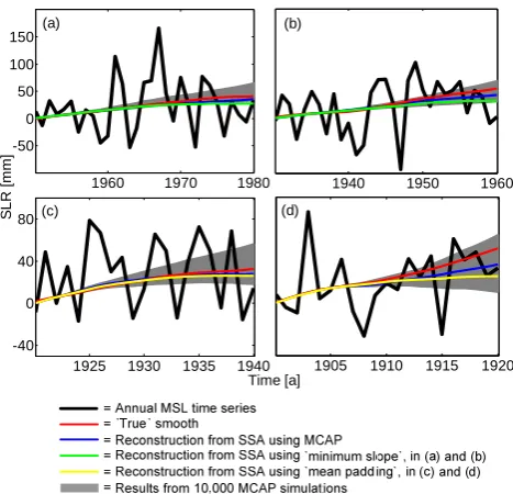
Fig. 3. Comparison of different methods for padding time series. Results are shown for the posterior boundary of truncated inter-vals of the annual MSL time series of the Cuxhaven gauge station: (a) the 1844 to 1980 interval, (b) the 1844 to 1960 interval, (c) the 1844 to 1940 interval and (d) the 1844 to 1920 interval.
The tide gauge records from Cuxhaven and Heligoland are used here to represent patterns of SLR in the German North Sea area. This seems to be justified, because both stations play an important role for sea level observation in the Ger-man North Sea and different authors proved that a very small number of long and high-quality tide gauge records capture the variability found from a considerably larger number of stations (e.g., Holgate, 2007). To compare the estimated pat-terns of SLR for the North Sea area to global patpat-terns of SLR, a worldwide sea level reconstruction published by Church and White (2006) is analysed using the presented methods. A recently updated version of the reconstruction, providing data from 1870 to 2007, is available from the homepage of the Permanent Service of Mean Sea Level (PSMSL).
3 Results
Before the results from both, the selected sea level time se-ries from the North Sea and the worldwide sea level recon-struction are presented in detail, the efficiency of the MCAP approach is demonstrated. Figure 3 shows the results for truncated intervals of the Cuxhaven annual MSL time series. The estimated smooth providing the smallest MSE, the re-sults from 10 000 MCAP simulations and the “true” smooth are calculated and compared in the figure. In addition, two simpler approaches for padding climate time series intro-duced by Mann (2004), namely the “minimum slope” and the “mean padding” approach are included for comparison
T. Wahl et al.: On analysing sea level rise in the German Bight since 1844 175
18
1960 1970 1980 -50
0 50 100 150
Time [a]
SL
R
[
m
m
]
1940 1950 1960
1925 1930 1935 1940 -40
0 40 80
1905 1910 1915 1920
(a) (b)
(c) (d)
504
Fig. 3. Comparison of different methods for padding time series. Results are shown for the
505
posterior boundary of truncated intervals of the annual MSL time series of the Cuxhaven
506
gauge station: (a) the 1844 to 1980 interval, (b) the 1844 to 1960 interval, (c) the 1844 to
507
1940 interval and (d) the 1844 to 1920 interval.
508
509
500 400 300 200 100
0.46 0.47 0.48
k
(t) [-]
Month [number] MEAN | 1-a sliding window
95% confidence bound of first window Exceedance rate < 0.6. Time series is stationary.
1000 800 600 400 200
MEAN | 1-a sliding window
95% confidence bounds of first window
Month [number] Exceedance rate < 0.6. Time series is stationary
510
Fig. 4. Results of the sliding-window test on stationarity applied to the monthly k-factor time
511
series of the Heligoland tide gauge (a) and the Cuxhaven tide gauge (b).
512
513
Fig. 4. Results of the sliding-window test on stationarity applied to the monthly k-factor time series of the Heligoland tide gauge (a) and the Cuxhaven tide gauge (b).
purposes. The “minimum slope” approach used in the most recent IPCC assessment (Trenberth et al., 2007) is included in Fig. 3a and b. The “mean padding” approach, also used in the IPCC assessment by Jansen et al. (2007) is included in Fig. 3c and d. Mann (2008) argues that both approaches are tending to artificially suppressing the trends near the bound-aries.
The results show that there is always a difference be-tween the estimated and the “true” smoothes. Especially for the 1844 to 1920 interval the “true” smooth clearly sug-gests a stronger SLR than the estimated smoothes. In ad-dition, a positive acceleration of SLR is indicated by the “true” smooth. The latter is displayed by the MCAP results, whereas the results from using the “mean padding” approach indicate a negative acceleration. The SSA reconstructions using MCAP show better results than the reconstructions us-ing the paddus-ing approaches applied in the most recent IPCC assessment in all cases. Only the reconstruction using “mini-mum slope” for the 1844 to 1980 interval slightly exceeds the shaded band resulting from 10 000 MCAP simulations. All the other reconstructions and the “true” smoothes proceed inside the band, which indicates the benefit of the approach. It should be noted, that the application of other methods for padding time series (e.g. Jevrejeva et al., 2006; Rahmstorf et al., 2007; Mann, 2008) lead to better results than the two methods used here for comparison purposes. Especially the “adaptive” approach introduced by Mann (2008) results in a very data adaptive smooth as the name indicates. But neither this one, nor any of the other methods allows the quantifica-tion of uncertainties near the boundaries due to the padding. In the following, the results from analysing the entire record sets of the Cuxhaven tide gauge and the Heligoland tide gauge are presented. Figure 4 shows the results of the sliding-window test on stationarity applied to the monthly k-factor time series. The latter were estimated for the periods providing high resolution data (see Sect. 2). From 20 000 Monte-Carlo simulations it was found that exceedance rates of the 95% confidence bounds of up to 60% are possible with stationary time series. Thus, both time series are found to be stationary from the sliding-window test as well as from the
Kolmogorov-Smirnov test. The k-factor time series of the Cuxhaven station (Fig. 4b) shows some irregularities at the end of the 1930s and in the 1940s (month numbers 250 to 400), which is probably an effect of the interruption of mea-sures (first of all dredging) in the estuary during and after the Second World War. Former studies suggest that the accu-racy of the k-factor improves in proportion to the resolution in time (Wahl et al., 2008). After the k-factor was found to be stationary for both stations, the mean is calculated for the period of 2000 to 2008 for the Heligoland station and for the period of 1998 to 2008 for the Cuxhaven station. Those pe-riods provide sea level data with a resolution in time of one minute. The estimated mean is 0.4783 for the Heligoland station, which equals a difference between MSL and MTL of about 5 cm. The mean k-factor for the Cuxhaven station is es-timated to 0.4685, which equals a difference between MSL and MTL of about 9 cm. The lower k-factor for the Cux-haven station clearly illustrates that the tide curve is subject to stronger deformations near the coastline due to shallow water effects.
The mean k-factor is used to correct the available MTL data from 1990 to 1999 for the Heligoland station and from 1844 to 1917 for the Cuxhaven station. Figure 5 shows the resulting monthly and annual MSL time series together with a fitted second order polynomial function providing the smallest MSE of the considered parametric approaches mentioned in Sect. 2. The Heligoland station shows a significant positive acceleration of 0.18±0.05 mm a−2 (two times the quadratic coefficient of the second order polyno-mial fit), a linear long-term trend of 1.85±0.42 mm a−1for the entire period and a linear trend of 8.50±2.32 mm a−1
176 T. Wahl et al.: On analysing sea level rise in the German Bight since 1844
1840 1860 1880 1900 1920 1940 1960 1980 2000 2020 -600
-400 -200 0 200 400 600 800
SL
R
[
m
m
]
Time [a] -600
-400 -200 0 200 400 600 800
S
L
R
[
mm]
514
Fig. 5.
Monthly and annual MSL time series for the Heligoland tide gauge (a) and the
515
Cuxhaven tide gauge (b) and results from parametric fitting.
516
Fig. 5. Monthly and annual MSL time series for the Heligoland tide gauge (a) and the Cuxhaven tide gauge (b) and results from parametric fitting.
2008. The linear trends for the period covered by both tide gauge records (1953 to 2008) are almost equal, which indi-cates the quality of the data. Furthermore, conspicuous high or low annual MSL values in general occur at both gauges at the same time. For example the low value for the year 1996, due to offshore winds and very little precipitation and runoff, or the high value for the year 1967, a year with many storm surges. The trend found for the twentieth century from the Cuxhaven time series differs slightly from that found by Woodworth et al. (2009b). He derived a linear trend of 1.4±0.2 mm a−1 from investigating a large number of tide gauges around the UK. The trends estimated for the short pe-riod from 1993 to 2008 are more than two times the trend found from global altimetry data for almost the same period (Beckley et al., 2007). This is an interesting result, but 16 years are a very short period to analyse high variability sea level time series as found in the German North Sea region.
The results for the non-linear data adaptive smoothing us-ing SSA with an embeddus-ing dimension of 11 years for the Heligoland time series and of 33 years for the Cuxhaven time series and the resulting annual rates of SLR are shown in Fig. 6. The results from the Cuxhaven station (Fig. 6c and
0 100 200 300
S
L
R
[mm]
(c)
1840 1860 1880 1900 1920 1940 1960 1980 2000 2020 -2
0 2 4 6
Time [a]
Ra
te
s of
S
L
R
[mm/a
]
(d) 0 100 200 300
SL
R
[
m
m
]
-2 0 2 4 6
Ra
te
s o
f
SL
R
[
m
m
/a
]
(a)
(b)
517
Fig. 6.
Results from non-linear smoothing using SSA in combination with MCAP and annual
518
rates of SLR estimated as the first deviation of the reconstruction providing the smallest MSE
519
for the Heligoland MSL time series ((a) and (b)) and the Cuxhaven MSL time series ((c) and
520
(d)).
521
522
0 50 100 150 200
SL
R
[
m
m
]
1860 1880 1900 1920 1940 1960 1980 2000 2020 1
2 3
Time [a]
Ra
te
s
o
f
SL
R
[
m
m
/a
]
(b) (a)
= Annual MSL time series
= Reconstruction from SSA providing the smallest MSE = Reconstructions from 10,000 MCAP simulations
523
Fig. 7.
Results from non-linear smoothing using SSA in combination with MCAP and annual
524
rates of SLR estimated as the first deviation of the reconstruction providing the smallest MSE
525
for a worldwide sea level reconstruction from 1870 to 2007.
526
Fig. 6. Results from non-linear smoothing using SSA in combi-nation with MCAP and annual rates of SLR estimated as the first deviation of the reconstruction providing the smallest MSE for the Heligoland MSL time series (a and b) and the Cuxhaven MSL time series (c and d).
d) point to a period of strong positive acceleration of SLR at the end of the 19th century, to a negative acceleration in sub-sequent years and to a period of almost no SLR around the 1970s with subsequent positive acceleration. High rates are observed for the period around 1900 and the highest rates of about 5 mm a−1are estimated for the year 2000. The inflec-tion point at the end of the 19th century is remarkably close to observed inflection points around 1880 at the Liverpool tide gauge (Woodworth, 1999) and around 1890 at the Brest tide gauge (W¨oppelmann et al., 2006).
The post 1970 acceleration is approved by the results from analysing the shorter MSL time series of the Heligoland sta-tion (Fig. 6a and b). The observed rates around 2000 from the Heligoland sea level time series are even higher than those found from the Cuxhaven time series, but clearly decrease in the recent years. Note that the annual rates were estimated from the SSA reconstruction providing the smallest MSE and that the uncertainties increase near the boundaries.
The results from analysing the recently updated global sea level reconstruction of Church and White (2006) are shown
T. Wahl et al.: On analysing sea level rise in the German Bight since 1844 177
20
0 100 200 300
S
L
R
[mm]
(c)
1840 1860 1880 1900 1920 1940 1960 1980 2000 2020 -2
0 2 4 6
Time [a]
Ra
te
s of
S
L
R
[mm/a
]
(d) 0 100 200 300
SL
R
[
m
m
]
-2 0 2 4 6
Ra
te
s o
f
SL
R
[
m
m
/a
]
(b)
517
Fig. 6.
Results from non-linear smoothing using SSA in combination with MCAP and annual
518
rates of SLR estimated as the first deviation of the reconstruction providing the smallest MSE
519
for the Heligoland MSL time series ((a) and (b)) and the Cuxhaven MSL time series ((c) and
520
(d)).
521
522
0 50 100 150 200
SL
R
[
m
m
]
1860 1880 1900 1920 1940 1960 1980 2000 2020 1
2 3
Time [a]
Ra
te
s
o
f
SL
R
[
m
m
/a
] (b) (a)
= Annual MSL time series
= Reconstruction from SSA providing the smallest MSE = Reconstructions from 10,000 MCAP simulations
523
Fig. 7.
Results from non-linear smoothing using SSA in combination with MCAP and annual
524
rates of SLR estimated as the first deviation of the reconstruction providing the smallest MSE
525
for a worldwide sea level reconstruction from 1870 to 2007.
526
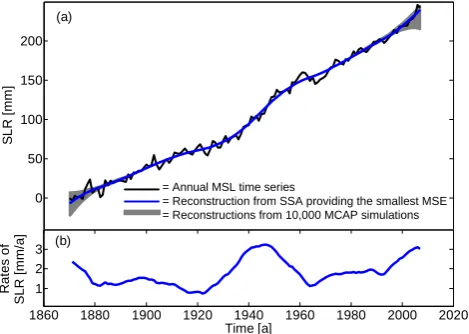
Fig. 7. Results from non-linear smoothing using SSA in combi-nation with MCAP and annual rates of SLR estimated as the first deviation of the reconstruction providing the smallest MSE for a worldwide sea level reconstruction from 1870 to 2007.
in Fig. 7. The time series provides data from 1870 to 2007. Thus, an embedding dimension of 28 years has been used for the SSA analysis. The smoothed time series shows remark-ably different patterns of SLR than the sea level time series from the German North Sea area. A positive acceleration oc-curred at the end of the 1930s, leading to high rates of SLR around 1940. A following negative acceleration led to low rates for the period after 1960 and rates are increasing again in the recent years.
Figure 8 clearly approves the existence of different pat-terns of SLR. It shows the difference 1 between the esti-mated annual rates of SLR for the Cuxhaven station (Fig. 6d) and the annual rates of SLR estimated from the global re-construction (Fig. 7b). The resulting time series highlights a stronger SLR in the German North Sea area for a period covering some decades at the end of the 19th century and the beginning of the 20th century and for another period cover-ing the last ten to fifteen years. For both periods the annual rates of SLR in the German North Sea area are found be up to 3 mm a−1higher than those estimated from a global sea
level reconstruction.
The correlation coefficient between the annual rates of SLR from the Cuxhaven station and the Heligoland station is found to ber=0.71 for the overlapping period from 1953 to 2008. The correlation between the annual rates of SLR from the Cuxhaven station and the annual rates estimated from the global sea level reconstruction is comparably weak. The cor-relation coefficient for the overlapping period from 1870 to 2007 is found to ber=0.33.
21
527
1860 1880 1900 1920 1940 1960 1980 2000 2020 -2
-1 0 1 2 3 4
Time [a]
[mm
/a
]
528
Fig. 8.
Difference
Δ
for the period of 1870 to 2007 between the annual rates of SLR estimated
529
from the Cuxhaven MSL time series and the annual rates of SLR estimated from a global sea
530
level reconstruction.
531
532
Fig. 8. Difference1for the period of 1870 to 2007 between the annual rates of SLR estimated from the Cuxhaven MSL time se-ries and the annual rates of SLR estimated from a global sea level reconstruction.
4 Conclusions and outline
In this paper, advanced methods to generate and analyse mean sea level time series are introduced. The presented modification of the k-factor method and the MCAP approach for padding non stationary sea level time series including un-certainty assessment contribute to overcome an existing lack of knowledge in analysing mean sea level time series, espe-cially in shallow seas. The results from analysing the avail-able data sets from two relevant tide gauges in the German North Sea highlight a post 1970 acceleration of SLR, which has not been reported before and which has obviously de-clined in recent years. The comparison between the Ger-man North Sea sea level time series and a global sea level reconstruction clearly reveals the existence of different pat-terns of SLR. A stronger SLR in the German North Sea area is detected for a period covering some decades starting at the end of the 19th century and for another period covering the last ten to fifteen years. However, coastal structures along the German North Sea coastline are well-conditioned and to some extend prepared for an expected SLR. In addition, the sea level is part of a complex system undergoing natural vari-ability and there are still considerable uncertainties in the re-sults.
Nevertheless, the study also indicates the necessity of fur-ther research in the field of sea level analysis and observa-tion. Uncertainties might be reduced by applying the re-sults of GPS measurements to improve the rates of vertical land movements considered in the sea level analyses (e.g. W¨oppelmann et al., 2007, 2009). Furthermore, a reduction of variability of the time series will result in an error reduc-tion. This might be done by considering more high qual-ity MSL time series from German North Sea tide gauges or by quantifying the impacts of stochastic meteorological pro-cesses such as wind setup or air pressure. All of the men-tioned work areas are subject to actual scientific efforts in Germany. More and more tide gauges are equipped with GPS by the Federal Agency of Hydrology (BfG, Koblenz).
178 T. Wahl et al.: On analysing sea level rise in the German Bight since 1844 A time consuming digitisation exercise is going on and
par-tially fulfilled at the University of Siegen. This is to allow the consideration of more high quality MSL time series to improve the results presented in this paper, e.g. by estimating a synthetic time series for the entire German North Sea area. The impact of wind set up and air pressure will be quantified in close cooperation with oceanographers from the Federal Maritime and Hydrographic Agency (BSH, Hamburg).
Finally, the presented results highlight the need for fur-ther research to improve regional climate models or regional sea level projections respectively. It is shown that regional patterns of SLR in the German North Sea area are not con-sistent with global patterns of SLR. Thus, the consideration of global SLR scenarios, as published for example by the IPCC, for regional planning purposes must be denoted as an interim solution. The results presented in this paper and the results expected after finishing the digitisation exercise will contribute to the verification of models for the German North Sea area.
Acknowledgements. We highly acknowledge the German Coastal Engineering Research Council (KFKI) and the German Federal Ministry of Education and Research (BMBF) for providing the opportunity to overcome an existing lack of knowledge in the field of mean sea level research in Germany by funding the research project “AMSeL – Mean Sea Level and Tidal Analysis at the German North Sea Coastline”. Thanks to Sylvin M¨uller-Navarra from the BSH in Hamburg for his professional comments on our work and to the anonymous reviewer helping to improve the quality of this paper.
Edited by: T. Glade
Reviewed by: S. M¨uller-Navarra and another anonymous referee
References
Beckley, B. D., Lemoine, F. G., Luthcke, S. B., Ray, R. D., and Zelensky, N. P.: A reassessment of global and regional mean sea level trends from TOPEX and Jason-1 altimetry based on revised reference frame and orbits, Geophys. Res. Lett., 34, L14608, doi:10.1029/2007GL030002, 2007.
Box, G. E. P. und Jenkins, G. M.: Time Series Analysis- forecasting and control, Holden-Day, London, 1976.
Chen, H. L. and Rao, A. R.: Testing Hydrologic Time Se-ries for Stationarity, J. Hydrologic Eng., 7(2), 129–136, doi:10.1061/(ASCE)1084-0699(2002)7:2(129), 2002.
Church, J. A. and White, N. J.: A 20th century acceleration in global sea-level rise, Geophys. Res. Lett., 33, L01602, doi:10.1029/2005GL024826, 2006.
Church, J. A., White, N. J., Aarup, T., Wilson, S. W., Woodworth, P. L., Domingues, C. M., Hunter, J. R., and Lambeck, K.: Under-standing global sea levels: past, present and future, Sustain. Sci., 3(1), 9–22, doi:10.1007/s11625-008-0042-4, 2008.
Dietrich, G.: Ozeanographisch-meteorologische Einfl¨usse auf Wasserstands¨anderungen des Meeres am Beispiel der Pegel-beobachtungen von Esbjerg, Die K¨uste, 2/2, 130–157, 1954.
F¨uhrb¨oter, A. and Jensen, J.: S¨akular¨anderungen der mittleren Tide-wasserst¨ande in der Deutschen Bucht, Die K¨uste, 42, 78–100, 1985.
Ghil, M., Allen, M. R., Dettinger, M. D., Ide, K., Kondrashov, D., Mann, M. E., Robertson, A. W., Saunders, A., Tian, Y., Varadi, F., and Yiou, P.: Advanced spectral methods for climatic time series, Rev. Geophys., 40(1), 1003, doi:10.1029/2000RG000092, 2002.
G¨onnert, G., Isert, K., Giese, H., and Pl¨uß, A.: Charakterisierung der Tidekurve, Die K¨uste, 68, 101–141, 2004.
Golyandina, N., Nekrutkin, K., and Zhigl¨ei`ıavskiæi, A. A.: Anal-ysis of time series structure, SSA and related techniques, Chap-man & Hall/CRC (Monographs on statistics and applied proba-bility, 90), Boca Raton, Florida, 2001.
Grinsted, A., Moore, J. C., and Jevrejeva, S.: Reconstructing sea level from paleo and projected temperatures 200 to 2100 AD, Clim. Dynam., published online first, doi:10.1007/s00382-008-0507-2, 2009.
Holgate, S. J.: On the decadal rates of sea level change dur-ing the twentieth century, Geophys. Res. Lett., 34, L01602, doi:10.1029/2006GL028492, 2007.
Holgate, S. J., Jevrejeva, S., Woodworth, P. L., and Brewer, S. C.: Comment on: “A Semi-Emprical Approach to Projecting Future Sea-Level Rise”, Empirical, Science, 317(5846), 1866– 1867, doi:10.1126/science.1140942, 2007.
Jansen, E., Overpeck, J., Briffa, K. R., Duplessy, J.-C., Joos, F., Masson-Delmotte, V., Olago, D., Otto-Bliesner, B., Peltier, W. R., Rahmstorf, S., Ramesh, R., Raynaud, D., Rind, D., Solom-ina, O., Villalba, R., and Zhang, D.: Palaeoclimate, in: Cli-mate Change 2007: The Physical Science Basis, Contribution of Working Group I to the Fourth Assessment Report of the In-tergovernmental Panel on Climate Change, edited by: Solomon, S., Qin, D., Manning, M., Chen, Z., Marquis, M., Averyt, K. B., Tignor, M., and Miller, H. L., Cambridge University Press, Cambridge, United Kingdom and New York, NY, USA, 2007. Jensen, J. and Mudersbach, C.: Zeitliche ¨Anderungen in den
Wasserstandszeitreihen an den Deutschen K¨usten, in: Berichte zur Deutschen Landeskunde, Themenheft: K¨ustenszenarien, Band 81, Heft 2, pp. 99–112, edited by: Glaser, R., Schenk, W., Vogt, J., Wießner, R., Zepp, H., und Wardenga, U., Selbstverlag Deutsche Akademie f¨ur Landeskunde e.V., Leipzig, 2007. Jevrejeva, S., Grinsted, A., Moore, J. C., and Holgate, S.: Nonlinear
trends and multiyear cycles in sea level records, J. Geophys. Res., 111, C09012, doi:10.1029/2005JC003229, 2006.
Jevrejeva, S., Moore, J. C., Grinsted, A., and Woodworth, P. L.: Recent global sea level acceleration started over 200 years ago?, Geophys. Res. Lett., 35, L08715, doi:10.1029/2008GL033611, 2008.
Lassen, H.: ¨Ortliche und zeitliche Variationen des Meeresspiegels in der s¨ud¨ostlichen Nordsee, Die K¨uste, 50, 65–96, 1989. Lentz, H.: Fluth und Ebbe und die Wirkungen des Windes auf den
Meeresspiegel, Otto Meissner, Hamburg, 1879.
Mann, H. B.: Nonparametric Test Against Trend, Econometrica, Journal of the Econometric Society, 13, 245–259, 1945. Mann, M. E.: On smoothing potentially non-stationary
cli-mate time series, Geophys. Res. Lett., 31, L07214, doi:10.1029/2004GL019569, 2004.
Meehl, G. A., Stocker, T. F., Collins, W. D., Friedlingstein, P., Gaye, A. T., Gregory, J. M., Kitoh, A., Knutti, R., Murphy, J. M., Noda, A., Raper, S. C. B., Watterson, I. G., Weaver, A. J., and Zhao, Z.-C.: Global Climate Projections, in: Climate Change 2007: The Physical Science Basis, Contribution of Working Group I to the Fourth Assessment Report of the Intergovernmental Panel on Climate Change, edited by: Solomon, S., Qin, D., Manning, M., Chen, Z., Marquis, M., Averyt, K. B., Tignor, M., and Miller, H. L., Cambridge University Press, Cambridge, United Kingdom and New York, NY, USA, 2007.
Mudersbach, C. and Jensen, J.: Non-stationarities in time series and its integration in extreme value statistics for risk management is-sues, Proc. of the 31st Int. Conf. on Coastal Engineering (ICCE), Hamburg, Germany, 2008.
M¨uller-Navarra, S. H. and Giese, H.: Improvements of an empirical model to forecast wind surge in the German Bight, DHZ, 51(4), 385–405, 1999.
Peltier, W. R.: Global Glacial Isostasy and the Surface of the Ice-Age Earth: The ICE-5G(VM2) model and GRACE, Ann. Rev. Earth. Planet. Sci., 32, 111–149, doi:10.1146/annurev.earth.32.082503.144359, 2004.
Pugh, D.: Changing Sea Levels: Effects of Tides, Weather and Cli-mate, 265 pp., Cambridge Univ. Press, New York, 2004. Rahmstorf, S.: A Semi-Empirical Approach to Projecting
Future Sea-Level Rise, Science, 315(5810), 368–370, doi:10.1126/science.1135456, 2007.
Rahmstorf, S., Cazenave, A., Church, J. A., Hansen, J. E., Keel-ing, R. F., Parker, D. E., and Somerville, R. C. J.: Recent Cli-mate Observations Compared to Projections, Science, 316, 709, doi:10.1126/science.1136843, 2007.
Rohde, H.: Die Pegel auf Helgoland, Die K¨uste, 49, 125–141,1990. Sch¨one, T., Sch¨on, N., and Thaller, D.: IGS Tide Gauge Benchmark Monitoring Pilot Project (TIGA): scientific benefits, J. Geodesy, 83(3/4), 249–261, doi:10.1007/s00190-008-0269-y, 2009. von Storch, H., Zorita, E., and Gonz´alez-Rouco, F.: Relationship
between global mean sea-level and global mean temperature in a climate simulation of the past millennium, Ocean Dynam., 58(3/4), 227–236, doi:10.1007/s10236-008-0142-9, 2008. T¨oppe, A. and Brockmann, T.: Tidewasserst¨ande am Pegel
Benser-siel seit 1825. Mitteilungen des Leichtweiss-Instituts f¨ur Wasser-bau, H. 120, Braunschweig, 1992.
Trenberth, K. E., Jones, P. D., Ambenje, P., Bojariu, R., Easterling, D., Klein Tank, A., Parker, D., Rahimzadeh, F., Renwick, J. A., Rusticucci, M., Soden, B., and Zhai, P.: Observations: Surface and Atmospheric Climate Change, in: Climate Change 2007: The Physical Science Basis, Contribution of Working Group I to the Fourth Assessment Report of the Intergovernmental Panel on Climate Change, edited by: Solomon, S., Qin, D., Manning, M., Chen, Z., Marquis, M., Averyt, K. B., Tignor, M., and Miller, H. L., Cambridge University Press, Cambridge, United Kingdom and New York, NY, USA, 2007.
Van Gelder, P. H. A. J. M., Mai, C. V., Wang, W., Shams, G., Ra-jabalinejad, M., and Burgmeijer, M.: Data management of ex-treme marine and coastal hydro-meteorological events, J. Hyd. Res., 46(2), 191–210, 2008.
Wahl, T., Jensen, J., and Frank, T.: Changing Sea Level and Tidal Dynamics at the German North Sea Coastline, Proc. of the Coastal Cities Summit 2008 – Values and Vulnerabilities, St. Pe-tersburg, Florida, USA, 2008.
White, N. J., Church, J. A., and Gregory, J. M.: Coastal and global averaged sea level rise for 1950 to 2000, Geophys. Res. Lett., 32, L01601, doi:10.1029/2004GL021391, 2005.
Woodworth, P. L.: High waters at Liverpool since 1768: the UK’s longest sea level record, Geophys. Res. Lett., 26(11), 1589–1592, 1999.
Woodworth, P. L., White, N. J., Jevrejeva, S., Holgate, S. J., and Gehrels, W. R.: Evidence for the accelerations of sea level on multi-decade and century timescales, Int. J. Climatol., 29(6), 777–789, doi:10.1002/joc.1771, 2009a.
Woodworth, P. L., Teferle, F. N., Bingley, R. M., Shennan, I., and Williams, S. D. P.: Trends in UK mean sea level re-visited, Geophys. J. Int., 176(22), 19–30, doi:10.1111/j.1365-246X.2008.03942.x, 2009b.
W¨oppelmann, G., Pouvreau, N., and Simon, B.: Brest sea level record: A time series construction back to the early eighteenth century, Ocean Dynamics, 56(5–6), 487–497, doi:10.1007/s10236-005-0044-z, 2006.
W¨oppelmann, G., Martin-Miguez, B., Bouin, M.-N., and Altamimi, Z.: Geocentric sea-level trend estimates from GPS analyses at relevant tide gauges world-wide, Global Planet. Change, 57, 396–406, 2007.
W¨oppelmann, G., Letetrel, C., Santamaria, A., Bouin, M.-N., Collilieux, X., Altamimi, Z., Williams, S. D. P., and Martin-Miguez, B.: Rates of sea-level change over the past century in a geocentric reference frame, Geophys. Res. Lett., 36, L12607, doi:10.1029/2009GL038720, 2009.