PIC 16F877A BASED IMPLEMENTATION OF FUZZY CONTROL
ALGORITHM FOR SPLIT AIR-CONDITIONING SYSTEM
C.B.Patil1, S. R. Potdar2 & R.R.Mudholkar3
1.INTRODUCTION
US Energy Information Administration (EIA) has reported that energy demand for space cooling is growing rapidly in India and all around the world, because of rising prosperity of mankind. Concurrently due to global warming, cooling degree days per year are increasing notably in the world, which further demands energy for space cooling. The current scenario reveals an exponential increase in use of room air conditioning. Among the various air conditioning systems, split air-conditioning units are generally used for small and medium scale offices and residential buildings.
Basically Air-Conditioning Systems are non-linear in which classical controllers such as ON/OFF and PID controllers are used. ON/OFF controller has simple structure and low initial cost. However it is more expensive due to their low energy efficiency. PID controller tends to be complex structure and initial cost is more. But, efficiency is more as compared to ON/OFF Controller. However PID Controller is set to operate at designed thermal loads, while actual thermal loads are time varying and depend on the environmental factors like outside weather conditions and number of occupants in the building. One way to overwhelm this is to use of Fuzzy Logic Controller, because it has ability to tackle multi-parameters, besides non-linear behavior of a system can be easily handled through fuzzy inference [1]. Many researchers are working on energy saving by applying different strategies on different parts of air conditioning unit. According to A. Benamer and D. Clodic, up to 40% energy saving is possible with variable speed compressor as compared to fixed speed compressor at lower heat loads [2]. Hu and Huang presented water cooled air conditioner that uses cellulose pads as a filling material of cooling tower. They showed that water cooled condenser results in decreasing the power consumption and improvement in COP significantly [3]. Amr O. Elsayed investigated that a condenser air flow can reduce about 10% in compressor power consumption [4].
2.SYSTEMIMPLEMENTATION
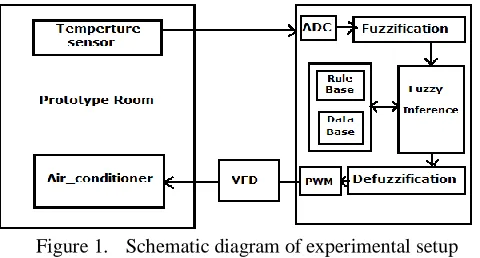
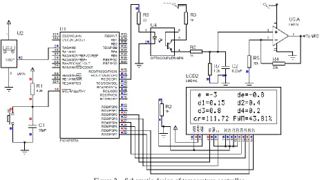
A schematic diagram of experimental setup is as shown in figure 1 and schematic design of temperature controller in figure 2.
Figure 1. Schematic diagram of experimental setup
1
Department of Electronics, D. K. A. S. C. College, Ichalkaranji, Maharashtra, INDIA-416115, (Affiliated to Shivaji University, Kolhapur, Maharashtra)
2
Department of Physics, Arts, Science and Commerce College, Rahata, Maharashtra, INDIA-423107
3
Department of Electronics, Shivaji University, Kolhapur, Maharashtra, INDIA-416004
International Journal of Latest Trends in Engineering and Technology
Vol.(9)Issue(2), pp.087-094
DOI: http://dx.doi.org/10.21172/1.92.15
e-ISSN:2278-621X
Figure 2. Schematic design of temperature controller
An isolated prototype room of dimension „2ft * 3ft * 4ft‟ made from thermocol with thickness 0.038m is considered inside which an evaporator unit of split AC is mounted. Split AC has various components for vapor compression cycle: a compressor, a condenser, an evaporator, metering device and fans. IC LM 35 sensor is used to sense the room temperature, which outputs an analog voltage. The analog output of sensor is given to ADC of PIC micro-controller, where it is converted into digital signal using scaling factor. The converted digital output is compared with set temperature value and accordingly an error signal is generated. The error signal is given as input to Fuzzy Inference System (FIS) implemented in PIC 16F877A microcontroller through C-code. FIS will then produce a crisp (count) value based on the control knowledge impersonated in the rule base. Depending upon count value micro-controller generates a Pulse Width Modulated (PWM) signal. The PWM signal is converted to proportional dc voltage in the range 0-10V with op-amp configured in non-inverting amplifier mode with gain of 2. The output of op-amp amplifier is fed to VFD (Variable Frequency Drive) which drives the compressor accordingly. In turn the evaporator temperature is changed and the system set in loop in maintaining the set temperature. The system simulink model in which, the Fuzzy Logic Controller modulates the ambiance of Air conditioned prototype room is shown in figure 3[5].
Figure 3. MATLAB simulink model of plant having prototype room and air conditioner with fuzzy logic controller
C.B.Patil, S. R. Potdar & R.R.Mudholkar 089
3.FUZZYLOGICCONTROLLER
Basically two types of Fuzzy Inference Systems (FIS), „Mamdani‟ and „Takagi-Sugeno‟ are used in control applications. They differ in compilation of output. Mamdani Fuzzy Controller has three stages of operations: fuzzification, fuzzy inference and defuzzification. In present system, Mamdani Fuzzy Controller is being used for fuzzy inference.
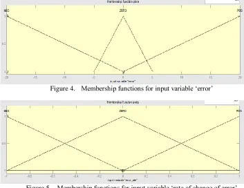
The FLC employed has two input fuzzy variables: error (e) and rate of change of error (de), one output fuzzy variable: count (u). The error is the difference between reference (set) value and current (measured) value of air temperature of room and rate of change of error is the rate of change between current error and previous error in time interval of 5 seconds. The count means a value in the range 0 to 255 that decides the duty cycle of PWM signal. The universe of discourse for (e) is -200C to +200C, for (de) is -10C to +10C, for (u) is 0 to 255. The input variable error (e) is partitioned into three fuzzy sets viz. NEGATIVE (N), ZERO (Z), POSITIVE (P), the input variable rate of change of error (de) is partitioned into three fuzzy sets viz. NEGATIVE (N), ZERO (Z), POSITIVE (P) and output variable count (u) is partitioned into three fuzzy sets viz. LOW (L), MED (M), HIGH (H) using triangular Membership functions. Fuzzy membership functions after tuning being applied are shown in figure 4, 5 and 6. The surface view of these variables is as shown in figure 7.
Figure 4. Membership functions for input variable „error‟
Figure 5. Membership functions for input variable „rate of change of error‟
Figure 7. Surface view for input error (e) and rate of change of error (de) and output count(c)
3.1 Fuzzification-
In this process, the degree of membership of particular fuzzy set for the input variables is calculated using the following formulae:
a) Triangular Membership Function- This MF is defined as,
Alternative expression obtained by min and max operations is follows: Triangle(x; a, b, c) = max(min((x-a)/(b-a), (c-x)/(c-b)),0)
Where the parameters „a‟, „b‟ and „c‟ are the x-coordinates of the three corners of the triangular MF. b) Trapezoidal Membership Function -
This MF is defined as,
Alternative expression obtained by min and max operations is follows: Trapezoid(x; a, b, c, d) = max (min ((x-a) / (b-a), 1, (d-x) / (d-c)), 0)
Where the parameters „a‟, „b‟, „c‟ and„d‟ are the x-coordinates of the four corners of the trapezoidal MF.
(a) (b)
Figure 8. Types of Membership functions (a) Triangular (b) Trapezoidal
The fuzzification process is illustrated as follows:
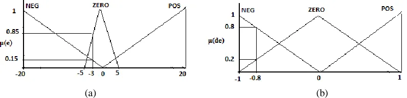
If error is -3 then the degree of memberships for input variable error (e) is calculated as shown in figure 9(a).
(a) (b)
C.B.Patil, S. R. Potdar & R.R.Mudholkar 091
Degree of membership for NEGATIVE fuzzy set (d1) = μN(e) triangle = 0-(-3)/0-(-20) = 3/20 = 0.15 Degree of membership for ZERO fuzzy set (d2) = μZ(e)triangle = -3-(-5)/0-(-5) = 2/5 = 0.4
If rate of change of error is -0.8 then the degree of memberships for input variable rate of change of error (de) is calculated as shown in figure 9(b).
Degree of membership for NEGATIVE fuzzy set (d3) = μN(de) triangle = 0-(-0.8)/0-(-1) = 0.8/1 = 0.8 Degree of membership for ZERO fuzzy set (d4) = μZ(de)triangle = -0.8-(-1)/0-(-1) = 0.2/1 = 0.2
3.2 Fuzzy inference-
In this process the degree of membership for each linguistic input term triggers the implication and derives a aggregated fuzzy output set. This task can be accomplished by referring to the data base, knowledge base and reasoning process. Reasoning process activated for priori formulated control laws relate the fuzzy input to fuzzy output from system behavioral knowledge as follows –
Rule 1: IF (error is NEG) and (rate rate of change of error is NEG) THEN count is HIGH Rule 2: IF (error is NEG) and (rate rate of change of error is ZERO) THEN count is HIGH Rule 3: IF (error is NEG) and (rate rate of change of error is POS) THEN count is HIGH Rule 4: IF (error is ZERO) and (rate rate of change of error is NEG) THEN count is MEDIUM Rule 5: IF (error is ZERO) and (rate rate of change of error is ZERO) THEN count is MEDIUM Rule 6: IF (error is ZERO) and (rate rate of change of error is POS) THEN count is LOW Rule 7: IF (error is POS) and (rate rate of change of error is NEG) THEN count is LOW Rule 8: IF (error is POS) and (rate rate of change of error is ZERO) THEN count is LOW Rule 9: IF (error is POS) and (rate rate of change of error is POS) THEN count is LOW
Rule 1 implies that the frequency of PWM signal generated is high, which delivers high voltage to VFD that drives the compressor with high speed of about 1150 rpm.
Rule 5 suggests that the frequency of PWM signal generated on PIC controller delivers a medium voltage, so that compressor rotates with medium speed of about 575 rpm.
Rule 9 infers that the frequency of PWM signal generated is very small, which drives the compressor with speed of about 64 rpm.
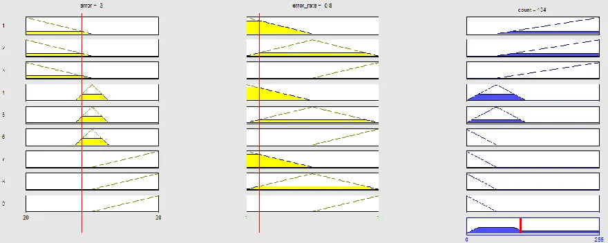
rules are to be evaluated to compute the degree of satisfaction to MF (LOW, MEDIUM, HIGH) of the output (count) pertaining to the degree of membership of the input variables. If error (e) = -3 and rate of change of error (de)= -0.8 only four rules get fired. The fuzzy Inference process is illustrated as shown in figure 10.
Rule 1: IF (e is NEG) (degree of 0.15) and (de is NEG) (degree of 0.8) THEN count is HIGH (degree of 0.15) (AND) Rule 2: IF (e is NEG) (degree of 0.15) and (de is ZERO) (degree of 0.2) THEN count is HIGH (degree of 0.15) (AND) Rule 4: IF (e is ZERO) (degree of 0.4) and (de is NEG) (degree of 0.8) THEN count is MEDIUM (degree of 0.4) (AND) Rule 5: IF (e is ZERO) (degree of 0.4) and (de is ZERO) (degree of 0.2) THEN count is MEDIUM (degree of 0.2)(AND) Since it is two input system with AND operator, the MF of the output will have the degree which is less among the memberships of input.
3.3 Defuzzification:
In this process from the aggregated fuzzy output, a crisp or numeric output value is calculated. There are numerous variants of the defuzzification procedure, such as Center of Gravity (COG), Centre of Sums (COS), Mean of maxima (MOM), First of maxima, Last of maxima, Weighted Average Method (WA). In present study the Weighted Average Method is used which can be represented mathematically as follows:
Where n = number of rules fired
= height of the rth clipped output fuzzy set. = Peak values of the rth clipped output fuzzy set.
Referring to the figure 9 the resulting fuzzy output at the end of the inference is converted into crisp value as follows:
0.15*255 0.4*58
(
) 111.72
0.15 0.4
c
The percentage PWM is calculated as follows:
*100
111.72*100
%
(
) (
) 43.81%
255
255
cr
pwm
4. ‘C’PROGRAMMODULE
// fuzzy implementation//
if((e<-20 ) && (de>=-1 && de<=0)) //CASE 1: e represents error and de represents error rate
{ cr=255;} // pwm with 100 % duty cycle
else if((e<-20 ) && (de>0 && de<=1)) //CASE 2
{ cr=255;} // pwm with 100 % duty cycle
else if((e>=-5 && e<=0) && (de>=-1 && de<=0)) //CASE 5 {d1=(0-e)/20; // μN(e)triangle
d2= (e+5)/5; // μZ(e)triangle
d3=(0-de)/1; // μN(de)triangle
d4=(de+1)/1; // μZ(de)triangle
if (d1<=d3) {a1= d1;} else {a1= d3;} if (d1<d4) { b1= d1;} else {b1= d4;} if(a1>=b1) {m3=a1;} else {m3=b1;} if (d2<=d3) {c1= d2;} else {c1= d3;} if (d2<d4) {e1= d2;} else {e1= d4;} if(c1>=e1) {m2=c1;} else {m2=e1;}
C.B.Patil, S. R. Potdar & R.R.Mudholkar 093
5.RESULTANDDISCUSSION
Figure 11. simulated results for Room-temperature, DoM, Crisp value, PWM value on Real_PIC simulator
The C-code being executed in Real-PIC simulator for three different situations and the results are as shown in figure 11. It is observed that when the room temperature is 30 0C which is above set point, the generated crisp value is 127.5, which produces the PWM wave of 50% duty cycle. When the room temperature is 23 0C, the generated crisp value is 111.72, which produces the PWM wave of 43.81% duty cycle. For room temperature of 16 0C which is below set point, the generated crisp value is 17.55, which produces the PWM wave of 6.8% duty cycle. This shows that duty cycle of PWM signals changes according to the error and rate of change of error.
In order to observe the performance of Fuzzy Logic Controller embedded in PIC, a set temperature value of 20 0C was given and the room temperature was logged. The data collected is plotted as shown in figure12. The MATLAB_Simulink model of plant has been executed and the result plotted is shown in figure 12. The computer simulation and experimental results are comparable which implicates the validity of the outcome. The little differences in parameter values are observed because of thermal mass effect that causes time lag in experimental readings which is not considered in computer simulation.
Figure 12. Variation in Room _Temperature for different controllers
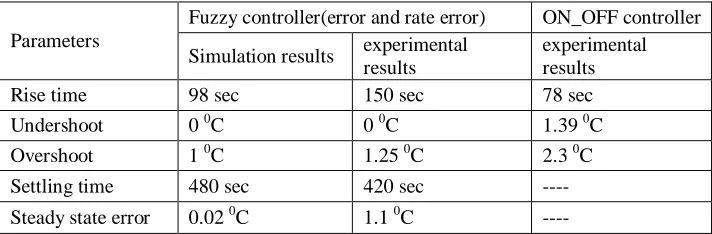
Also the ON-OFF controller embedded in PIC was executed for same set point value of 20 0C. The result plotted is shown in figure 12. Because of continuous turn ON and OFF mechanism and overshooting the power consumption is increasing significantly which further makes wear and tear of air conditioner parts noticeably. The comparison between Fuzzy controller and ON_OFF controller results are tabulated in Table 1. It is observed that ON-OFF controller reaches the set value earlier than Fuzzy controller but with considerable overshoots and undershoots.
Table -1 Performance Matrix for simulated and experimental results
Parameters
Fuzzy controller(error and rate error) ON_OFF controller
Simulation results experimental results
experimental results
Rise time 98 sec 150 sec 78 sec
Undershoot 0 0C 0 0C 1.39 0C
Overshoot 1 0C 1.25 0C 2.3 0C
Settling time 480 sec 420 sec ----
6. CONCLUSION
The fuzzy algorithm to control the air conditioner temperature has been successfully designed and implemented in 8-bit PIC 16F877A microcontroller. With few rules, a control is being accomplished in a stand-alone hardware. Hence the design approach presented in this paper is cost effective. Further energy consumption is reduced greatly in fuzzy logic controller than ON-OFF controller, addition to prolong the wear and tear of air conditioner. Hence there is significant improvement in the performance of the Air conditioning system.
7.REFERENCES
[1] Rachana R. Mudholkar et al, “Genetic Tuning of Fuzzy Inference System for Furnace Temperature Controller”, (IJCSIT) International Journal of
Computer Science and Information Technologies, Vol. 6 (4) , 2015, 3496-3500.
[2] A.Benamer and D. Clodic, “Comparison of Energy Efficiency Between Variable and Fixed Speed Scroll Compressors in Refrigeration System”,
Proceedings of technological innovations in refrigeration in air conditioning and in the food industry into third millennium, June, 1999, pp.1-8.
[3] S.S. Hu and B.J. Huang, “Study of a High Efficiency Residential Split Water-Cooled Air Conditioner”, Applied Thermal Engineering, 25, 2005, pp.
1599–1613.
[4] Amr O. Elsayed1, Abdulrahman S. Hariri1 “Effect of Condenser Air Flow on the Performance of Split Air Conditioner”, World Renewable Energy
Congress 2011-Sweden, 8-13 May 2011.
[5] C.B.Patil et.al, “Thermal modeling of air-conditioned prototype room using Matlab- Simulink”, International Journal of Engineering Science and