Abstract—Different designs of manufacturing systems are adopted in industry today. A good manufacturing design should be flexible to compensate for uncertainties such as demand fluctuations and machine breakdowns. A new conceptual manufacturing system called Multi-Channel Manufacturing (MCM) is expected to provide flexibility and efficiency under uncertainties. This paper proposes an integration model that considers capacity decisions and manufacturing system design. There are two objectives in this research. The first objective is to create a robust manufacturing system design over the planning horizon. The robust design considers the changes in the capacity decisions and in the operation strategies. The second objective is to show that robust MCM design is superior to other robust manufacturing system design based on the cost evaluation in this research. The results indicate that MCM design is often chosen to minimize cost. The results also demonstrate that different operation strategies are used to minimize cost for compensating the demand uncertainty.
Index Terms—Multi-channel manufacturing, MCM, manufacturing systems, robust design, capacity planning.
I. INTRODUCTION
In industry today, flexibility is an important issue. A company should be able to provide enough flexibility to operate in uncertain environments, for example in a situation with fluctuating demand. To provide enough flexibility, the design strategy over the planning horizon of the manufacturing system must be carefully considered. Usually, the planning horizon is categorized into long-range planning, medium-range planning, and short-range planning. Each of the three planning horizons contains its own set of decisions. Long-range planning activities include business forecasting, product and sales planning, production planning, resource requirements planning, and financial planning. Medium-range planning activities include distribution requirements planning, demand management, master production scheduling, rough cut capacity planning, material requirements planning, and capacity requirements planning. Short-range planning activities involve the final assembly scheduling, production activity control, and purchase planning and control. In designing a manufacturing system, integrating all the different design strategies would create the best manufacturing system, but such integration is impossible to implement. It is often difficult to integrate the decisions that have different time horizons.
To analyze a new way to design manufacturing systems, it is important and pertinent to clearly address the reasons to integrate or not to integrate different planning decisions.
Manuscript received October 29, 2015; revised December 30, 2015. Ping-Yu Chang is with the Department of Industrial Engineering and Management, Ming Chi University of Technology, New Taipei City, 24311, Taiwan (e-mail: [email protected]).
Manufacturing systems design implies allocating resources, such as personnel, facilities, equipment, and inventory, so that the planned products and services are available when needed. Usually, prior facility decisions limit the capacity available and should be updated when the demand and the material requirement significantly change. To provide more flexibility in the manufacturing system, the design should span the active planning horizon and should provide changes in the facility design and capacity requirements.
In reviewing the research, production planning is usually considered after the manufacturing system design is known. Production planning and inventory have an effect on the material requirement planning and may have an effect on the capacity when the demand changes. However, it is hard to integrate production planning into the stage of designing the manufacturing system. The manufacturing system design is long-range planning and is updated infrequently when more capacity is needed. Production planning is performed after the manufacturing system design is known and more frequently in response to customer demand.
Capacity planning is an important decision in manufacturing system design. A robust manufacturing system design should be able to provide a plan for updating the capacity requirement over the planning horizon. The plan should also provide information on changing the channel design, since changing the channel design would affect the queueing time and the throughput time of the products. Changing the channel design includes machine relocation and/or adding more machines. Machine relocation involves moving a machine to another channel or forming a new channel to increase the flexibility of the system. Adding machines increases the flexibility of the system but also increases the machine cost. The decision for adding more machines will depend on the tradeoff between the machine cost and WIP cost.
A formulation is proposed here to determine a robust manufacturing system design for MCM. The formulation attempts to minimize the total cost, which is defined as the total WIP cost plus the machine relocation cost and the machine cost. The WIP cost is evaluated using the queueing approximations. By minimizing the total cost in the objective function, the capacity requirement planning and the manufacturing design are obtained from the formulation. The capacity decisions such as whether to buy some more machines to meet the demand at different time periods can also be made by solving these models.
II. LITERATURE REVIEW
Meller [9] introduced the design of the MCM system with two mixed integer programming (MIP) optimization models. The models considered the channel design considering the
Robust Hybrid Manufacturing System Design
cost, the budget, and the required channel coefficients. In his models, the demand is fixed and is only considered for a single period. In many situations, manufacturing system design covering multiple time periods is needed. This design must consider the overall cost while determining the best capacity and production plans. In order to design the system, different planning strategies such as capacity planning and production planning should be considered for formulating the optimization model.
From the literature reviews of manufacturing system design, only a few papers were found that addressed integrating the design strategies for robust manufacturing system. Abdelmola et al. [1] optimized the productivity of CM systems using a two-stage model. The first stage was to design the manufacturing cells and the part families for CM systems. The capacity requirements are formulated as the available machine time in this optimization model. The second stage was to optimize the productivity of the designed CM system. The results of a numerical example showed that the productivity improved for CM and that the cost is reduced through the first stage. They also mentioned that the proposed model had deficiencies with respect to large scale problems. A good heuristic should be provided to achieve shorter computational time in solving large scale problems. A disadvantage of their model is that the planning horizon is only for a single period ([4]-[6]).
Askin and Mitwasi [2] and Askin and Standridge [3] integrated the facility layout with process selection and capacity planning. They presented a mathematical formulation to show the integration of facility layout, process selection, flow planning and capacity planning. Their formulation showed some interesting ideas for integrating the design strategies. Again, a disadvantage of their formulation is that their planning horizon is only for a single period.
Peters and McGinnis [10] introduced a new planning problem that provides a bridge from strategy to capacity by focusing on the configuration of key manufacturing resources. Furthermore, they present a single period approximation, which provides analytical insights in finding the best system design to meet the production requirements. They defined the system design as the configuration of production facilities that are focused factories with dedicated lines, general factories with lines capable of producing multiple products, and some hybrid combination. Two solutions approaches, lagrangean dual and branch-and-bound, are proposed and examined in their research. The results show that two proposed solutions approaches provide good results and acceptable computational times.
Peters and McGinnis [11] addressed the strategic facility configuration and assignment of products to facilities for a pure focused strategy over multiple time periods. They described the strategic planning problem, introduced and developed a formulation for the product assignment/reassignment phenomenon, and provided a framework for its analysis that illustrated several insights. Moreover, they developed a procedure to determine the minimum capacity solution for the case of a pure focused strategy. The procedure provides insights and foundations to a multi-commodity network based procedure for determining the optimal set of product assignments and reassignments for
a given set of facilities and capacity levels. They proved the constraint matrix is totally unimodular and showed that realistic size problems are solvable (less than 5 minutes) using standard solution techniques ([7], [8]).
Schaller et al. [12] presented a mathematical formulation to integrate cell design and production planning. They generate a list of possible cell formations as input to the mathematical formulation. The mathematical formulation then selects the cell from the list to minimize the production cost, inventory cost, and backorder cost. They provided several heuristic procedures and compared the results of heuristic procedures to the lower bound obtained from the linear programming relaxation. Although they provide the mathematical formulation for multiple period planning horizons, the disadvantage is that the design of the manufacturing system is selected from the predetermined list of cell formations. Additionally, their manufacturing system design procedure didn’t allow changes in capacity levels over time as product demand changes ([13], [14]).
Reviews of the manufacturing system design literature show that there have been only a few attempts to integrate the manufacturing system design with production planning and capacity planning. Similarly, relatively few papers provide the integrating system design strategies for multiple period planning horizons. To approach the robust MCM system design, the ideas from previous research such as creating the system design at one stage and achieving the maximum productivity at the second stage ([1]) or creating the list of potential cell designs and integrating the list with production planning considerations ([12]), should be carefully considered and expanded. Furthermore, this research attempts to integrate the manufacturing system design and capacity planning over multiple time periods and the methodology is discussed further in Section III.
III. METHODOLOGY
There are three pieces of information in the manufacturing system design provided in the optimization model. The first piece of information is the number of channels and the channel design. Once a machine is bought and the channel is opened, the machine is assigned to a channel. The machine assignment criteria are the machine requirements of the product and the CC value of the product. The second piece of information is the machine relocation. To achieve better performance in terms of better throughput, the channel design might be changed by relocating the machines. The information of the machine relocation is provided by the formulation. The third piece of information is the CC value of the product and the channels assigned for the product. The formulation will assign different number of channels and different channels for the products in different categories. Before introducing the formulations, notation is listed here.
i = index for the products (i = 1,…,I),
j = index for the machine types (j = 1,…,J),
m, k = index for the channels (m, k =1,…,K),
p = index for the time period (p=1,…,P),
A = set of class A-products,
B = set of class B-products,
p j
U = upper bound on number of machine type j in period
p,
p ij
Lf = lower bound on fraction of machine type j’s capacity
required by product i at period p. This value can be determined by total capacity requirement for the demand lower bound of product i at period p / total machine capacity available for machine type j at period p.
p ij
Uf = upper bound on fraction of machine type j’s
capacity required by product i at period p. This value can be determined by total capacity requirement for the demand upper bound of product i at period p / total machine capacity available for machine type j at period p
wij = 1, if product i requires machine j ( wij = 1 if Lfijp > 0 );
0, otherwise,
cj = cost of one copy of machine type j, p
i
CC = CCi of product i in period p, p
A
CC = lower bound on CCi for class A-products in period
p, p B
CC = lower bound on CCi for class B-products in period
p, p C
CC = lower bound on CCi for class C-products in period
p, p i
CW = WIP cost of product i in period p, p
i
WIP = WIP of product i in period p,
Mj = relocation cost of machine type j.
the decision variables are presented as follows.
xjkp = number of machines of type j assigned to channel k in
period p, p ik
z = 1, if product i is assigned to channel k in period p; 0, otherwise,
p k
O = 1, if channel k is opened in period p; 0, otherwise. Note that the value for CCAp, CCBp, and CCCp will be
predefined.
The objective function (1) is to minimize the total cost. The total cost is the summation of the machine cost, the WIP cost, and the machine relocation cost.
P p J j K k jkp K
k jkp j P p J j K
k jkp jkp j P p I i p i p i x x C x x M WIP CW Min
1 1 1 , 1 1
1 1 1 , 1 1 1 ) ( | | : (1) Constraint (2) makes sure that there are enough machines
in the channel for the products that are assigned to this channel. . , , , ) ( 1 p k j x I w
z ij jkp
I
i p
ik
(2)
Constraint (3) is the demand constraint. It ensures that machine types are available with enough capacity to produce the minimum level of demand.
. , , 1 1 1 p j Uf x Lf I i p ij K k jkp I i p
ij
(3)
Constraint (4) makes sure that no machine will be assigned to the channel if the channel is not open.
. , , ,
)
(O j k p
M
xjkp kp (4) Constraint (5) sets the lower bound for the number of
channels, and constraint (6) sets the CCi value for the product. , , , 1 p A CC
O pA
K
k p
k
(5)
. , , 1 p i z CC K k p ik p
i
(6)
Constraints (7) – (9) set the lower bound on the CCi value
for products in categories A, B, and C. , ,
, i A p
CC
CC p
A p
i (7) ,
,
, i B p
CC
CC p
B p
i (8) .
,
, i C p
CC
CC pC
p
i (9) Constraint (10) defines the WIP value. This value is a function of the number of machines and the products assigned to the channel. Moreover, this value will be evaluated using the queueing approximations.
). , , , , ,
(i j k p x z f
WIP p
ik jkp p
i (10) Constraint (11) is the integer constraint on the machine assignment variables. Constraints (12) and (13) are the binary constraints on the product assignment and channel selection variables.
, , ,
, k j p
Z
xjkp
(11) , , , , } 1 , 0
{ i k p
zikp (12) . , , } 1 , 0
{ k p
Op
k (13) In the formulations, the term WIPip represents the average
WIP in the system for product i in period p and is evaluated by the queueing approximations from the analytical models. The reason for using the analytical models is the advantage of running time. The simulation models may provide results that include more realistic assumptions than the analytical models but will take longer time to construct and run. This time difference shows the advantage of using analytical models since repeated evaluations will need to be made. To implement the analytical models, the manufacturing system design, the product process plan, the operation strategies (i.e., batch size), the material handling time, and the expected demand information for each product are required.
TABLEI:FACTORIALS OF EXPERIMENTAL DESIGN
# of vehicles
Batch Size\scheduling
rules
# of channels
1 2 3 CM
1
10 FIFO SPT FIFO SPT FIFO SPT FIFO SPT
30 FIFO SPT FIFO SPT FIFO SPT FIFO SPT
50 FIFO SPT FIFO SPT FIFO SPT FIFO SPT
2
10 FIFO SPT FIFO SPT FIFO SPT FIFO SPT
30 FIFO SPT FIFO SPT FIFO SPT FIFO SPT
50 FIFO SPT FIFO SPT FIFO SPT FIFO SPT
3
10 FIFO SPT FIFO SPT FIFO SPT FIFO SPT
30 FIFO SPT FIFO SPT FIFO SPT FIFO SPT
50 FIFO SPT FIFO SPT FIFO SPT FIFO SPT
Once estimated, the WIP cost is incorporated into the objective function (the summation of material handling cost, the machine cost, the WIP cost, and the machine relocation cost) for evaluating the manufacturing system designs. Overall, the WIP cost contributes to the total cost function for evaluating the manufacturing system designs while the inputs are from the optimization and simulation models. Moreover,
the discussion for the solution methodology in the next section will provide more insight to the usage of the WIP cost.
IV. RESULTS AND COMPARISONS
The applicability of the developed models is tested on an example derived from Abdelmola et al. (1998). This manufacturing system consists of eleven parts and seven machines. The manufacturing system evaluation is in terms of the decision making for different manufacturing systems to achieve minimum cost over multiple time periods. To evaluate the manufacturing systems, WIP level is obtained using the analytical queueing models. The summation of WIP cost, machine cost, material handling vehicle cost, and machine relocation cost is evaluated to compare different manufacturing systems. The heuristic is implemented using AMPL, CPLEX (optimization model), and MATLAB (analytical models). The sensitivity analysis and results are discussed in the remainder of this section.
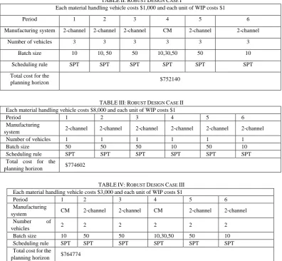
TABLEII:ROBUST DESIGN CASE I
Each material handling vehicle costs $1,000 and each unit of WIP costs $1
Period 1 2 3 4 5 6
Manufacturing system 2-channel 2-channel 2-channel CM 2-channel 2-channel
Number of vehicles 3 3 3 3 3 3
Batch size 10 10, 50 50 10,30,50 50 10
Scheduling rule SPT SPT SPT SPT SPT SPT
Total cost for the
planning horizon $752140
TABLEIII:ROBUST DESIGN CASE II Each material handling vehicle costs $8,000 and each unit of WIP costs $1
Period 1 2 3 4 5 6
Manufacturing
system 2-channel 2-channel 2-channel 2-channel 2-channel 2-channel
Number of vehicles 1 1 1 1 1 1
Batch size 50 50 50 10 50 10
Scheduling rule SPT SPT SPT SPT SPT SPT
Total cost for the
planning horizon $774602
TABLEIV:ROBUST DESIGN CASE III Each material handling vehicle costs $3,000 and each unit of WIP costs $1
Period 1 2 3 4 5 6
Manufacturing
system CM 2-channel 2-channel CM 2-channel 2-channel
Number of
vehicles 2 2 2 2 2 2
Batch size 10 50 50 10,30,50 50 10
Scheduling rule SPT SPT SPT SPT SPT SPT
Total cost for the
planning horizon $764774
Table II shows the total cost over the planning horizon when each material handling vehicle costs $1,000 and each unit of WIP costs $1. The cost for each period is the summation of machine cost, WIP cost, and material handling vehicle cost. The relocation cost in these results is assumed to be not significant when compared to other cost. If the
analysis is carried out to understand the effect of the number of material handling vehicles and WIP cost on the decisions. Sensitivity of the cost function is determined for three material handling vehicle cost levels ($1,000, $3,000, and $8,000) and five WIP cost levels ($1, $2, $5, $10, and $30).
The results show that the 2-channel MCM is preferred for most of the periods. Only in period four, CM is chosen but CM is cheaper than 2-channel MCM by only $0.3. The
results in Table V also show that three material handling vehicles and SPT rule are chosen in all six periods. As the cost of each vehicle increases, the number of material handling vehicles used in the manufacturing systems decreases. Tables III and IV give the cost in each period when the material handling vehicles cost $3000 and $8000, respectively.
TABLEV:ROBUST DESIGN CASE IV Each material handling vehicle costs $3,000 and each unit of WIP costs $2
Period 1 2 3 4 5 6
Manufacturing
system 2-channel 2-channel 2-channel CM 2-channel 2-channel Number of
vehicles 3 2 3 2 3 2
Batch size 10 50 50 10,30,50 50 10
Scheduling rule SPT SPT SPT SPT SPT SPT
Total cost for the
planning horizon $968475
TABLEVI:ROBUST DESIGN CASE V Each material handling vehicle costs $3,000 and each unit of WIP costs $5
Period 1 2 3 4 5 6
Manufactu
ring system 2-channel 2-channel
2-chann
el CM 2-channel 2-channel
Number of
vehicles 3 3 3 3 3 3
Batch size 10 10, 50 50 10,30,
50 50 10
Scheduling
rule SPT SPT SPT SPT SPT SPT
Total cost for the planning horizon
$1550700
TABLEVII:ROBUST DESIGN CASE VI Each material handling vehicle costs $3,000 and each unit of WIP costs $10
Period 1 2 3 4 5 6
Manufactu
ring system 2-channel 2-channel 2-channel CM 2-channel 2-channel Number of
vehicles 3 3 3 3 3 3
Batch size 10 10, 50 50 10,3
0,50 50 50
Scheduling
rule SPT SPT SPT SPT SPT SPT
Total cost for the planning horizon
$2541399
TABLEVIII:ROBUST DESIGN CASE VII Each material handling vehicle costs $3,000 and each unit of WIP costs $30
Period 1 2 3 4 5 6
Manufacturi
ng system 3-channel 3-channel 2-channel 3-channel 3-channel 3-channel Number of
vehicles 3 3 3 3 3 3
Batch size 30 50 10 10 50 50
Scheduling
rule SPT SPT SPT SPT SPT SPT
Total cost for the planning horizon
$6482508
manufacturing systems and operation rules may change. Furthermore, fewer material handling vehicles will be required for the manufacturing system and different batch size might be used for the manufacturing systems.
In Tables II, III, and IV, 3-channel MCM system is never chosen because of the high machine cost ($13,000) for adding an additional channel to the 2-channel MCM, even though, the WIP level of 3-channel MCM is less than the
WIP level of 2-channel MCM, CM or JS. If the WIP cost per unit is increased in the cost function, 3-channel might be favored. Sensitivity analysis is performed to understand the effect of WIP cost on the decisions. Sensitivity of the cost function is determined for five WIP levels ($1, $2, $5, $10, and $30) and shown in Tables IV, V, VI, VII, and VIII. The level for the cost of each material handling vehicle is $3,000.
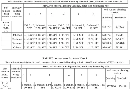
TABLEIX:ALTERNATIVE SOLUTION CASE I
Best solution to minimize the total cost (cost of each material handling vehicle: $3,000, each unit of WIP costs $1)
best solution
using heuristic
alternative solution
using simulation
MFG, # of material handling vehicles, Batch size, Scheduling rule
1 2 3 4 5 6
total cost for planning horizon
Queueing Simulation
Recall from Table 4.14
CM, 2, 10, SPT
2-channel, 2, 50, SPT
2-channel, 2, 50, SPT
CM, 2, (10, 30, 50), SPT
2-channel, 2, 50, SPT
2-channel, 2,
10, SPT $764774 $740233
Job shop 3, 10, SPT 3, 10, SPT 3, 10, SPT 3, 10, SPT 3, 10, SPT 3, 10, SPT $767773 $826187
2-channel 2, 50, SPT 2, 50, SPT 2, 50, SPT 2, 50, SPT 2, 50, SPT 2, 50, SPT $764775 $754863
3-channel 3, 50, SPT 3, 50, SPT 3, 50, SPT 3, 50, SPT 3, 50, SPT 3, 50, SPT $770806 $794178
Cellular 2, 50, SPT 2, 50, SPT 2, 50, SPT 2, 50, SPT 2, 50, SPT 2, 50, SPT $764917 $755169
TABLEX:ALTERNATIVE SOLUTION CASE II
Best solution to minimize the total cost (cost of each material handling vehicle: $8,000 and each unit of WIP costs $1)
best solution
using heuristic
alternative solution
using simulation
MFG, # of material handling vehicles, Batch size, Scheduling rule
1 2 3 4 5 6
total cost for planning horizon
Queueing Simulation
Recall from Table 4.13
2-channel, 1, 50, SPT
2-channel, 1, 50, SPT
2-channel, 1, 50, SPT
2-channel, 1, 10, SPT
2-channel, 1, 50, SPT
2-channel, 1, 10,
SPT $775906 $761988
Job shop 3, 50, SPT 3, 50, SPT 3, 50, SPT 3, 50, SPT 3, 50, SPT 3, 50, SPT $782773 $840187
2-channel 1, 50, SPT 1, 50, SPT 1, 50, SPT 1, 50, SPT 1, 50, SPT 1, 50, SPT $775906 $761988
3-channel 2, 10, SPT 2, 10, SPT 2, 10, SPT 2, 10, SPT 2, 10, SPT 2, 10, SPT $783917 $815065
Cellular 2, 10, SPT 2, 10, SPT 2, 10, SPT 2, 10, SPT 2, 10, SPT 2, 10, SPT $776917 $765169
The results show that increasing the cost of each unit of WIP will change the design and operation rules. As the WIP cost increases, the optimal solution tends to have more material handling vehicles. When the cost of each unit of WIP increases to $30, a 3-channel MCM system is chosen in the first period, since the WIP for 3-channel MCM is significantly less than the other manufacturing systems. In subsequent periods, the WIP reduction is not large enough to offset the machine cost so the 2-channel MCM is preferred. Clearly, the specific design will depend on the parameters for each situation.
The results shown in Tables II–VIII: are based on the assumption of no significant relocation cost for moving machines or changing configurations. However, changing the relocation cost will impact the decisions made. It is important to understand the impact of increasing the relocation cost on the choice of manufacturing systems and operation rules.
The results and analysis in Tables 2 - 8 show that MCM design becomes favored as the WIP cost and the relocation cost increase. However, the overall quality of solutions
provided by this heuristic is not known. Unfortunately, a good lower bound is not available, so an alternative solution approach using simulation is presented. The alternative solution provides the best design with minimum cost for JS, CM, and MCM. The alternative solution for the scenario in Table VI is shown in Table IX.
Table IX compares the cost for the best heuristic solution using simulation and queueing approximation. The cost for the best available solution using either the queueing approximation or the simulation dominate the other alternative solutions based on pure strategies. However, the cost for the best solution using simulation achieves a lower cost than the best solution using the queueing approximation. This result is the difference in accuracy of between the queueing approximation and the simulation in estimating WIP levels. However, the cost difference between the solutions is small, such that they are within 3.2% of one another.
manufacturing. The difference may be due to the design of the material handling system in the simulation models. The design of the material handling uses the SDS (smallest distance to station) rule and different distances between the machine centers are applied to different manufacturing system configurations. Because of these design concepts, the waiting time in the queue of material handling vehicles will be correlated, which results in the correlation in the queue length. To avoid the effect of these correlations, batch means are used to compute the simulation results in Tables 9 and 10. However, the simulation is only run until the demand for each period is satisfied and did not contain enough information to reduce the variance estimate. Examples with larger demands that can provide longer run times may mitigate the effect and should be included in further studies. Other queueing approximations to accurately estimate WIP will also improve this methodology and represent another potential area for further research.
Table X summarizes another example where each material handling vehicle costs $8,000. The results for the robust solution estimated with both simulation and queueing still dominate the alternative pure strategies solutions. This result confirms the conclusion that the heuristic will provide good solutions and can be used as a basis for further research.
V. CONCLUSION AND FUTURE RESEARCH
In this paper, a mixed integer programming model is proposed. In particular, a comprehensive optimization model is proposed in this research that integrates capacity decisions with the manufacturing system design to gain insight into MCM robustness. To implement the model, the WIP levels are obtained through queueing approximations to evaluate the cost function of a manufacturing system configuration. The cost function consists of the WIP cost, machine requirement cost, machine relocation cost, and material handling cost. The results indicate that MCM system design is often chosen to minimize cost. The results also demonstrate the sensitivity of the solution to changes in the WIP cost per unit and relocation cost.
The robustness of MCM is addressed in this research. A foundation is developed in this area, but clearly more work could be done. For example, the WIP level is obtained through a queueing approximation, which cannot be optimized directly in the optimization model. Different WIP approximations to account for more realistic scenarios will provide different solutions and may affect the robust design. Therefore, developing and evaluating a more accurate WIP
approximation should be an important topic for future research.
REFERENCES
[1] A. I. Abdelmola, S. M. Taboun, and S. Merchawi, “Productivity optimization of cellular manufacturing systems,” Computers and Industrial Engineering, vol. 35, pp. 403-406, 1998.
[2] R. G. Askin, and M. G. Mitwasi, “Integrating facility layout with process selection and capacity planning,” European Journal of Operational Research, vol. 57, pp. 162-173, 1992.
[3] R. G. Askin, and C. R. Standridge, Modeling and Analysis of Manufacturing Systems, John Wiley & Sons Inc., New York, 1993. [4] U. S. Karmarkar, “Lot sizes, lead times, and in-process inventories,”
Management Science, vol. 33, pp. 409-418, 1987.
[5] U. S. Karmarkar, S. Kekre, and S. Freeman, “Lot-sizing and lead time performance in a manufacturing cell,” Interfaces, vol. 15, pp. 1-9, 1985.
[6] A. Kavusturucu, and S. M. Gupta, “Manufacturing systems with machine vacations, arbitrary topology and finite buffers,” International Journal of Production Economics, vol. 58, pp. 1-15, 1999.
[7] A. M. Law, “Pitfalls in the simulation of manufacturing systems,”
Winter Simulation Conference Proceedings, Washington D.C., 539-542, 1986.
[8] R. Logendran, and D. Talkington, “Analysis of cellular and functional manufacturing systems in the presence of machine breakdown,”
International Journal of Production Economics, vol. 53, pp. 239-256, 1997.
[9] R. D. Meller, “White paper on multi-channel manufacturing,” Technical Report, Department of Industrial and Systems Engineering, Virginia Polytechnic Institute and State University, Blacksburg, 1998. [10] B. A. Peters, and L. F. McGinnis, “Strategic configuration of flexible assembly systems: A single period approximation,” IIE Transactions, vol. 31 issue 4, pp. 379-390, 1999.
[11] B. A. Peters, and L. F. McGinnis, “Modeling and analysis of the product assignment problem in single stage electronic assembly systems,” IIE Transactions, vol. 32, issue 1, pp. 21-31, 2000. [12] J. E. Schaller, S. S. Erenguc, and A. J. Vakharia, “A mathematical
approach for integrating the cell design and production planning decisions,” International Journal of Production Research, vol. 38, issue 16, 3953-3971, 2000.
[13] P. J. Schweitzer, “Maximum throughput in finite-capacity open queueing networks with product-form,” Management Science, vol. 24, pp. 217-223, 1977.
[14] T. Yang, and B. A. Peters, “Flexible machine layout design for dynamic and uncertain production environments,” European Journal of Operational Research, vol. 108, pp. 49-64, 1998.
Ping-Yu Chang is an assistant professor in the Department of Industrial Engineering and Management at Ming Chi University of Technology (MCUT), Taiwan. He received his master degree in manufacturing engineering at Syracuse University in 1996 and his Ph.D. degree in industrial engineering at Texas A&M University in 2002. His current research and teaching interests are in the supply chain and production management. In particular, he is interested in supply chain management, facility location, scheduling, and simulation modeling. Author’s formal