Empirical Analysis of Differential Evolution
Algorithm with Rotational Mutation Operator
Amit R. Khaparde
Department of Computer Science and Engineering GHRCE, RGCER, Nagpur, Maharashtra, India.
Dr. M. M. Raghuwanshi
Department of Computer Technology YCCE, Nagpur, Maharashtra, India
Dr. L. G. Malik
Department of Computer Science and Engineering GHRCE, Nagpur, Maharashtra, India.
Abstract - A New rotation mutation strategy in differential evolution is proposed. It uses the local information to rotate the trial vector in search space. It provides the exploration to search operator of differential evolution algorithm. It has been tested on 25 test function of CEC 2005 test suite. The results of proposed algorithm are compared with standard differential evolution. The results of proposed method are slightly better than standard differential evolution algorithm, in multi model problems.
Keywords – rotation , rotation matrix , multi-model functions.
I. INTRODUCTION
Finding the best solution from the set of feasible solution is called optimization. The optimization problems can be solved by using direct algorithms and stochastic algorithms. Evolutionary algorithms are meta-heuristics can be used to solve optimization problems. The entire evolutionary algorithm’s computational model mimics the evolutionary processes. The non-linear and non-differential continuous space optimization problems can be solved by heuristic methods. Differential evolution algorithm (DE) [1] is a good choice to solve these problems because it is very easy to use, robust, require few control parameter and automatically impart to parallel computation [2] [3][4] [5] . DE has high convergence speed as compare to other evolutionary algorithms. DE is very capable to solve engineering optimization problems [6]. Though there are very few control parameters but still the choosing the proper control parameters is difficult [7]. If the control parameter does not choose properly, then problem like premature convergence, stagnation [8] can occur and it give an undesirable results. Mutation strategy play a vital role in population evolution, the convergence nature of DE [9] and parameter setting [10] is affected by the type of mutation strategy. Lack of selection pressure in mutation strategies [11] during evolution can cause stagnation or premature convergence hence there must be a proper combination of exploration and exploitation during evolution. The performance of mutation strategies vary with the type of problem [12][13]. They have different parameter settings according to the problems [14] [15]. The rest of the paper is organized are as follows, Section I give the introduction of differential evolution algorithm. In section II discuss the related work in the field. Section III covers the proposed work. Experimental results and empirical analysis is in section IV. Section V is conclusion.
II. DIFFERENTIAL EVOLUTION ALGORITHM 1. Initialization of initial population
Differential evolutionary algorithm (DE) begins its process by randomly initializing the NP number of D dimensions vectors within a search space. They also know as genome / chromosomes. This vectors act as candidate solution for a given objective functions. Every cycle in DE can be consider as a generation, G= 1,2,3 ….. Gmax. Then any candidate solution at any generation can be denoted as :x i,g=[x1,g,x2,g,x3,g ……….xD,g]. There exists a lower and upper bound within search space for each parameter in the problem, let it can be denoted as :
Xmin=[X1,min,X2,min ……Xd,min] and Xmax=[X1,max,X2,max ……Xd,max]
The initial population (G=0) must cover the maximum range as much as possible between the lower and upper bound. This can be achieved by following equation :
X j,i,0= X j,min + rand [0,1] (X j,max - X j,min ) (1)
whereas xj,i,0 =jthcomponent of ithmember of population at 0thgeneration and xj,min and xj,min its respective lower and upper value. Generally variable bounds are used for population initialization (on safer side) but initialization is also possible without using variable bounds.
2. Mutation
Each point (individual) can be represented as vector in search space. In DE each parent vector of current generation is known as target vector. All individuals in current generation get a chance to become a target vectors. The
resultant vector obtain through mutation is known as donor vector. DE generates a donor vector by adding the
weighted difference between two population vectors to a third vector. For each target vector Xi, G, i = 1, 2, . . . NP, a mutant vector is generated as follows
Vi;G+1= Xr1;G + F * (Xr2,G - Xr3,G) (2) Whereas r1, r2, r3ɽ13are mutually different integers and )!ɽ>@known as scaling factor. The integer r1, r2 and r3 are randomly chosen. That to be different from the running index i. F is a real and constant factor which controls the amplification of the differential variation (xr2,G- xr3,G) .
3. Crossover
Each chromosome or solution in a population is a set or vector of D decision variables. Probability of crossover (CR) decides how many variables (out of D variables) in solution will change their value. For example if CR=0.6
then only 60% variables will change their value and 40% will remain unchanged.
It increases the diversity of the population. The parameters of mutated vector are mixed with the parameters of another predetermined vector, the target vector, to yield the so-called trial vector. This parameter mixing is referred as crossover. In crossover trial vector u i;G+1 = (u 1i,G+1, u 2i,G+1 . . . u Di;G+1) is formed . DE provides the two different type of crossovers binomial crossoverand exponential crossover. The binomial crossover can be define as :
U ji;G+1= V ji,G+1LIUDQGEM&5RUM UQEUL (3) X ji,GLIUDQGEM!&5DQGMUQEUL
j = 1, 2 . . . D. randb(j) is the jth evaluation of a uniformUDQGRP QXPEHU JHQHUDWRU ɽ > @&5 LV WKH FURVVRYHU
FRQVWDQWɽ>@UQEULLVDUDQGRPO\FKRVHQLQGH[ɽ«'ZKLFKHQVXUHVWKDW8i,G+1 gets at least one parameter from vi,G+1
4. Selection
To decide whether or not new vector should become a member of generation G+1, the trial vector Ui,G+1 is compared to the target vector Xi,G using the greedy criterion. If vector U i,G+1yields a smaller cost function value than X i,G, then X i,G+1is set to U i,G+1; otherwise, the old value Xi,G is retained
Ui,G if f(U i,GI;i,G)(4)
Xi,G+1= (4)
Xi,G else
Each population vector has to serve once as the target vector so that NP competitions take place in one generation. This process is continue until the stopping criteria is not meet
There are number of variants in DE. In order to represent the variants the following notation is used DE=x/y/z is Where as x: The vector to be mutated which currently can be “rand” (a randomly chosen population vector) or “best” (the vector of lowest cost from the current population).y: Number of difference vectors used. z: The crossover scheme.
Table 1: Variants of DE
Sr . No Strategy S r. No Strategy
1 DE/best/1/exp 6 DE/best/1/bin
2 DE/rand/1/exp 7 DE/rand/1/bin
3 DE/rand-to-best/1/exp 8 DE/rand-to-best/1/bin
4 DE/best/2/exp 9 DE/best/2/bin
5 DE/rand/2/exp 10 DE/rand/2/bin
III. RELATED WORK
The exploration at starting phase of evolution and exploitation during end of ending phase of evolution [16] , A new framework along with second enhance mutation operator [17] been used to ensure the trade-off between the exploration and exploitation is the phenomenon has increased the performance of SDE.
The new mutation scheme- DE/current-to-gr_best/1 [18] , is a variant of the classical DE/current-to-best/1 scheme which uses the best of a group of randomly selected solutions from current generation mutation, give the better exploration and recombination each mutant vector with one of the p top-ranked individuals from the current population ensure exploitation along with parameter adaption scheme enhance the performance of SDE. [19] use local search to update scaling factor of solution space to balance the exploration and exploitation, Asymmetric mutation operator [20] used different scaling factor to handle balance the exploration and exploitation. One of the advantage of SDE is that it is free from any PDF (probability density function), in order to balance exploration and exploitation , there are some mutation operator have used PDF like Gaussian PBX-alpha(GPBX-alpha) [21] , improved CRDE[22], co-evolutionary method to update scaling factor[23] ,GDDE[24] the main drawback of these methods are they incurred extra decision parameters and extra computation cost on DE.
IV. PROPOSED ALGORITHM
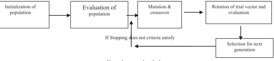
The mutation operation in differential evolution algorithm is rotation invariant but the crossover operator of differential evolution algorithm is not rotation invariant, hence some time DE does not give a desire results in complex optimization problems. Here, a new mutation scheme is incurred in standard differential evolution algorithm (SDE). The trial vector is rotated in search space using local information. The detail process is given in [25]. The process is shown in figure.
Figure 1. proposed method
In order to rotate the trial vector in the search space, the angle of rotation is require. It can be calculate by following methods :
I. Angle based upon the local information of given vector(Method 1)
. Initialization of
population Evaluation of population
Mutation & crossover
Rotation of trial vector and evaluation
II. Angle depend upon compliment based upon the local information (Method 2)
The opposition based learning rotate the individual in search space in angle of . The method is as follows:
a. Calculate vector by using method 1
b. Find the compliment of vector using opposition based learning rule.
III. Angle depend upon compliment based upon the angle of 360 degree
Angle = -
The process of rotation can be depicted in figure.
Figure 2. Method for rotation
IV. EXPERIMENTAL RESULTS AND DISCURSION
The performance of new rotation mutation scheme is tested on the all problems of CEC 2005 test suite [26]. Further the performance of suggested method is compared with standard differential evolution algorithms. The parameter setting for the experimentation is shown in the table 2.
Table 2:Parameter setting for DESBS
Sr. No. Parameter Values
1 Number of Variables (D) 5,10
2 Scaling Factor (F) 0.5
3 Crossover Rate (Cr) 0.9
4 Size of Initial Population (NP) 20 5 Maximum Function Evaluation (Max_Fev) 1000
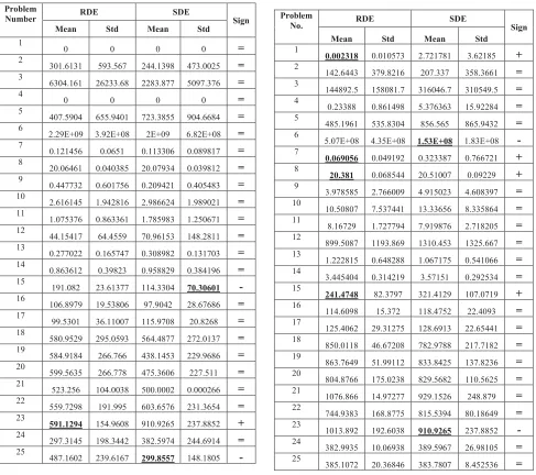
For all the problems algorithms are executed for 25 times. The performance of the each method is evaluated on bases of Minimum value of function. The wilcoxon rank sum test[27] is used to check the null hypothesis. The null hypothesis in each test is that “there no difference exists between the original SDE and the proposed mutation method . We mark the cases with “ + ” when the null hypothesis is rejected and the DESBS outperforms the other one in a statistically significant way, with “–” when the null hypothesis is rejected and the original SDE/variant of SDE is significantly better than the other, with “ = ” when the null hypothesis is accepted and no performance difference is significant.
Calculate rotation angle
Calculate rotation matrix using M by using Aguilera-Perez Algorithm[26]
Compute the rotating vector.
Evaluate the new rotated vector
Table 3. size of variable is 5 Table 4. size of variable is 10
As from table 3 and table 4 , when the number of variables are small that time SDE perform better as compare to proposed method whereas as the number of variable increases, the proposed method perform better than standard algorithm . most of the time both of algorithms are statically same ,I,e there is no any significant difference in the performance of both algorithms . In fact the proposed algorithm incurred the extra computation cost on the standard differential evolution algorithm.
IV.CONCLUSION
The new mutation strategy for mutation vector rotation has been proposed . it incurred extra computation cost on standard DE but as the number of variable increases it give the better performance as compare to standard differential evolution algorithm . although the experimentation is carry out on 5 and 10 number of variable , it is very early to say regarding the performance . the performance of proposed method in multi model functions is encouraging . tuning of control parameters is require.
Problem
Number RDE SDE Sign
Mean Std Mean Std
1
0 0 0 0 =
2
301.6131 593.567 244.1398 473.0025 = 3
6304.161 26233.68 2283.877 5097.376 = 4
0 0 0 0 =
5
407.5904 655.9401 723.3855 904.6684 = 6
2.29E+09 3.92E+08 2E+09 6.82E+08 = 7
0.121456 0.0651 0.113306 0.089817 = 8
20.06461 0.040385 20.07934 0.039812 = 9
0.447732 0.601756 0.209421 0.405483 = 10
2.616145 1.942816 2.986624 1.989021 = 11
1.075376 0.863361 1.785983 1.250671 = 12
44.15417 64.4559 70.96153 148.2811 = 13
0.277022 0.165747 0.308982 0.131703 = 14
0.863612 0.39823 0.958829 0.384196 = 15
191.082 23.61377 114.3304 70.30601 -16
106.8979 19.53806 97.9042 28.67686 = 17
99.5301 36.11007 115.9708 20.8268 = 18
580.9529 295.0593 564.4877 272.0137 = 19
584.9184 266.766 438.1453 229.9686 = 20
599.5635 266.778 475.3606 227.511 = 21
523.256 104.0038 500.0002 0.000266 = 22
559.7298 191.995 603.6576 231.3654 = 23
591.1294 154.9608 910.9265 237.8852 + 24
297.3145 198.3442 382.5974 244.6914 = 25
487.1602 239.6167 299.8557 148.1805
-Problem
No. RDE SDE Sign
Mean Std Mean Std
1
0.002318 0.010573 2.721781 3.62185 + 2
142.6443 379.8216 207.337 358.3661 = 3
144892.5 158081.7 316046.7 310549.5 = 4
0.23388 0.861498 5.376363 15.92284 = 5
485.1961 535.8304 856.565 865.9432 = 6
5.07E+08 4.35E+08 1.53E+08 1.83E+08 -7
0.069056 0.049192 0.323387 0.766721 + 8
20.381 0.068544 20.51007 0.09229 + 9
3.978585 2.766009 4.915023 4.608397 = 10
10.50807 7.537441 13.33656 8.335864 = 11
8.16729 1.727794 7.919876 2.718205 = 12
899.5087 1193.869 1310.453 1325.667 = 13
1.222815 0.648288 1.067175 0.541066 = 14
3.445404 0.314219 3.57151 0.292534 = 15
241.4748 82.3797 321.4129 107.0719 + 16
114.6098 15.372 118.4752 22.4093 = 17
125.4062 29.31275 128.6913 22.65441 = 18
850.0118 46.67208 782.9788 217.7182 = 19
863.7649 51.99112 833.8425 137.8236 = 20
804.8766 175.0238 829.5682 110.5625 = 21
1076.866 14.97277 929.1526 248.879 = 22
744.9383 168.8775 815.5394 80.18649 = 23
1013.892 192.6038 910.9265 237.8852 -24
382.9935 10.06938 389.5967 26.98105 = 25
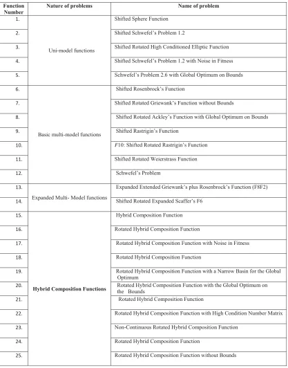
Table 5. Detail of the functions
Function Number
Nature of problems Name of problem
1.
Uni-model functions
Shifted Sphere Function
2. Shifted Schwefel’s Problem 1.2
3. Shifted Rotated High Conditioned Elliptic Function 4. Shifted Schwefel’s Problem 1.2 with Noise in Fitness
5. Schwefel’s Problem 2.6 with Global Optimum on Bounds
6.
Basic multi-model functions
Shifted Rosenbrock’s Function
7. Shifted Rotated Griewank’s Function without Bounds
8. Shifted Rotated Ackley’s Function with Global Optimum on Bounds
9. Shifted Rastrigin’s Function
10. F10: Shifted Rotated Rastrigin’s Function
11. Shifted Rotated Weierstrass Function
12. Schwefel’s Problem
13.
Expanded Multi- Model functions
Expanded Extended Griewank’s plus Rosenbrock’s Function (F8F2)
14. Shifted Rotated Expanded Scaffer’s F6
15.
Hybrid Composition Functions
Hybrid Composition Function
16. Rotated Hybrid Composition Function
17. Rotated Hybrid Composition Function with Noise in Fitness
18. Rotated Hybrid Composition Function
19. Rotated Hybrid Composition Function with a Narrow Basin for the Global Optimum
20. Rotated Hybrid Composition Function with the Global Optimum on the Bounds
21. Rotated Hybrid Composition Function
22. Rotated Hybrid Composition Function with High Condition Number Matrix 23. Non-Continuous Rotated Hybrid Composition Function
24. Rotated Hybrid Composition Function
REFERENCES
[1] R. Storn , K. Price “Differential Evolution – A Simple and Efficient Heuristic for Global Optimization over Continuous Spaces”.Journal of Global Optimization, pp, 341-359, 11: 341–359, 1997.
[2] R. Storn , K. Price “ Differential Evolution - A simple and efficient adaptive scheme for global optimization over continuous spaces”, TR-95-012. March, 1995.
[3] R. Storn “ System Design by Constraint Adaptation and Differential Evolution”,TR-96-039,November 1996. [4] K. Price, “Differential Evolution: A Fast and Simple Numerical Optimizer”,IEEE,1996.
[5] K. P. Wong, Z. Y. Dong, “Differential Evolution, an Alternative Approach to Evolutionary Algorithm”, ISAP, 2005.
[6] D. Karaboga, S. Okdem ,” A Simple and Global Optimization Algorithm for Engineering Problems: Di_erential Evolution Algorithm “,Turk J Elec Engin,, VOL.12, NO.1, 2004.
[7] R. Gamperle, S. Mu ller, P. Koumoutsakos,” A Parameter Study for Differential Evolution”, [8] J. Lampinen, I. Zelinka. ,”On Stagnation Of The Differential Evolution Algorithm,”
[9] G.Jeyakumar, C.Shanmugavelayutham,” Convergence Analysis Of Differential Evolution Variants On Unconstrained Global Optimization Functions “,International Journal of Artificial Intelligence & Applications (IJAIA), Vol.2, No.2, April 2011.
[10] K.V. Price, J. I. Rönkkönen,” Comparing the Uni-Modal Scaling Performance of Global and Local Selection in a Mutation-Only Differential Evolution Algorithm “ ,IEEE Congress on Evolutionary Computation, 2006.
[11] A.M. Sutton ,M. Lunacek , L. D. Whitley,” Differential Evolution and Non-separability: Using selective pressure to focus search “,GECCO’07, July 7–11, 2007.
[12] E. MezuraMontes, J. VelazquezReyes, Coello Coello,” A Comparative Study of Differential Evolution Variants for Global Optimization “,GECCO,2006.
[13] Wenyin Gong, Zhihua Cai,” An Empirical Study on Differential Evolution for Optimal Power Allocation in WSNs “ , International Conference on Natural Computation,2012.
[14] S. Chattopadhyay, S. Sanyal , A. Chandra,” Comparison of Various Mutation Schemes of Differential Evolution Algorithm for the Design of Lowpass FIR Filter “ ,International Conference on Sustainable Energy and Intelligent System,2011.
[15] Y. Ao, H. Chi,” Experimental Study on Differential Evolution Strategies “ , Global Congress on Intelligent Systems,2009.
[16] M.G. Epitropakis, V.P. Plagianakos, and M.N. Vrahatis,” Balancing the exploration and exploitation capabilities of the Differential Evolution Algorithm “,IEEE, 2008.
[17] C. Deng, B. Zhao, A. Deng ,R,Hu,” New Differential Evolution Algorithm with a Second Enhanced Mutation Operator”, IEEE, 2009. [18] Sk. Islam, S. Das, S. Ghosh, S. Roy, P. N. Suganthan, “An Adaptive Differential Evolution Algorithm With Novel Mutation and Crossover
Strategies for Global Numerical Optimization “IEEE TRANSACTIONS ON SYSTEMS, MAN, AND CYBERNETICS—PART B: CYBERNETICS, VOL. 42, NO. 2, APRIL 2012.
[19] F. Neri,V. Tirronen, T. Karkainen, “Enhancing Differential Evolution Frameworks by Scale Factor Local Search - Part II” ,IEEE,2009. [20] E. C. Shi, Hung Ham, J.. C.Y. Lai,”An Adaptive Differential Evolution with Unsymmetrical Mutation”.IEEE,2009.
[21] A. Nobakhti , H. Wang ,”Co-evolutionary Self-Adaptive Differential Evolution with a Uniform-distribution Update Rule “International Symposium on Intelligent Control,2006
[22] R.Zhou, J. Hao, H. Cao, H.Fan, ”An Empirical Study on Differential Evolution Algorithm and Its Several Variants”International Conference on Electronic & Mechanical Engineering and Information Technolog,2011
[23] Li Chen, L. Ding, ”An improved crowding-based differential evolutionfor multimodal optimization”,IEEE,2011.
[24] Radha Thangraj l, Millie Pantl, Ajith Abraham2, Kusum Deepl, Vaclav Snasee, ”Differential Evolution using a Localized Cauchy Mutation Operator”,IEEE,2010
[25] A.Khaparde, M. Raghuwanshi,L.Malik,”New Mutation Scheme in Differential Evolution Algorihm” ,ICBIM ,2016 [26] A.Aguilera,,R.Pérez-Aguila,”General n-Dimensional Rotations”WSCG'2004.