e-ISSN: 2278-067X, p-ISSN: 2278-800X, www.ijerd.com
Volume 13, Issue 9 (September 2017), PP.35-42
A Comprehensive Study Report on Load balancing Techniques in
Cloud Computing
1
st*Dr.Chinthagunta Mukundha,
2Nampally Venkatesh,
3Kamatagi Akshay
1Associate Professor, Dept of IT, Sreenidhi Institute of Science & Technology,Hyderabad, 2UG Schoolar, Dept of IT, Sreenidhi Institute of Science & Technology,Hyderabad, 3
UG Schoolar, Dept of IT, Sreenidhi Institute of Science & Technology,Hyderabad, Corresponding Author: *Dr.Chinthagunta Mukundha
ABSTRACT:
Cloud computing is emerging as a new paradigm for manipulating, configuring, and accessing large scale distributed computing applications over the network. Load balancing is one of the main Challenges in cloud computing which is required to distribute the workload evenly across all the nodes. Load is a measure of the amount of work that a computation system performs which can be classified as CPU load, network load, memory capacity and storage capacity. It helps to achieve a high user satisfaction and resource utilization ratio by ensuring an efficient and fair allocation of every computing resource. Proper load balancing aids in implementing fail-over, enabling scalability, over- provisioning, minimizing resource consumption and avoiding bottlenecks etc. This paper describes a survey on load balancing algorithms in cloud computing environment along with their corresponding advantages, disadvantages and performance metrics are discussed in detail.Keywords:
cloud computing, manipulating, memory capacity, provisioning, load balancing.I.
INTRODUCTION
Load balancing in clouds is a technique that distributes the excess dynamic local workload evenly across all the nodes. It is used for achieving a better service provisioning and resource utilization ratio, hence improving the overall performance of the system Incoming tasks are coming from different location are received by the load balancer and then distributed to the data center ,for the proper load distribution.
The aim of load balancing is as follows: To increase the availability of services To increase the user satisfaction To maximize resource utilization
To reduce the execution time and waiting time of task coming from different location. To improve the performance
Maintain system stability Build fault tolerance system Accommodate future modification
Challenges of Load Balancing
Overhead Associated: Determines the amount of overhead involved while implementing a loadbalancing system. It is composed of overhead due to movement of tasks, inter-process communication. Overhead should be reduced so that a load balancing algorithm performs well.
Throughput: It is the number of task executed in the fixed interval of time. To improve the performance of the system, throughput should be high.
Performance: It can be defined as the efficiency of the system. It must be improved.
Resource Utilization: Is used test the utilization of resources. It should be maximum for an efficient load balancing system.
Scalability: The quality of service should be same if the number of users increases. The more number of nodes can be added without affecting the service.
Response Time: Can be defined as the amount of time taken to react by a load balancing algorithm in a distributed system. For better performance, this parameter should be reduced.
Fault Tolerance: In spite of the node failure, the ability of an system to perform uniform load balancing. The load balancing is the best fault-tolerant technique.
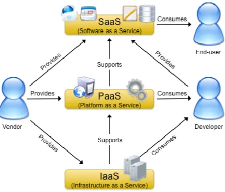
Fig : Cloud Computing Architecture
Virtualization:
Cloud computing uses virtualization as a base for provisioning services to the client. Multiple operating systems can be run on the single computer on the base of virtualization so utilization of resources is increased. For enhanced the productivity of server the hardware resources are combined. For the proper resource utilization the, computer architecture is uses software called Hypervisor. It is also called Virtual Machine Monitor (VMM) for running the multiple operating systems on the single host. Hypervisor provides the computing resources (memory, processor, and bandwidth) to the virtual machine. There are two types of virtualization in cloud computing.
Full Virtualization: In Full Virtualization, the entire installation of one computer is done on the other computer. So the functionality of the actual machine can also be available in virtual machine.
Para Virtualization: In Para Virtualization, multiple operating systems can be run on a single machine. Here all the functionalities are not fully available, rather than the services are provided in a partial manner.
II.
RELATED WORK
The cloud facility is a network of geographically distributed datacenters, each consisting of hundreds of servers. When a user submits a task (popularly known as cloudlet) it is handled by the datacenter controller. The Data Center Controller , uses a VmLoadBalancer to determine which VM should be assigned the next request for processing. The Vmloadbalancer can use the following algorithms for load balancing. • Round Robin - The datacenter controller assigns the requests to a list of VMs on a rotating basis. The first request is allocated to a VM picked randomly from the group and then the subsequent requests are assigned in a circular order. Once the VM is assigned a request, it is moved to the end of the list. Though the work load distributions between processors are equal but the job processing time for different processes are not same. So at any point of time some nodes may be heavily loaded and others remain idle.
Weighted Round Robin – It is the modified version of Round Robin in which a weight is assigned to each VM so that if one VM is capable of handling twice as much load as the other, the powerful server gets a weight of 2. In such cases, the Data Center Controller will assign two requests to the powerful VM for each request assigned to a weaker one. The major issue in this allocation is same as that of Round Robin that is it also does not consider the advanced load balancing requirements such as processing times for each individual requests .
Dynamic Round Robin - This algorithm mainly works for reducing the power consumption of physical machine. The two rules used by this algorithm is as follows:
i) If a virtual machine has finished its execution and there are other virtual machines hosted on the same physical machine, this physical machine will accept no more new virtual machine. Such physical machines are called to be in "retiring" state, i.e. when rest of the virtual machines finishes their execution, and then this physical machine can shut down.
Randomized – It randomly assigns the selected jobs to the available VM. The algorithm is very simple but it does not take into consideration whether the VM is overloaded or under loaded. Hence, this may result in the selection of a VM under heavy load and the job may require a long waiting time before being serviced.
Equally Spread Current Execution (ESCE) Algorithm - In this method the load balancer continuously scans the job queue and the list of virtual machines. If there is a VM available that can handle the request then the VM is allocated to that request . If there is an overloaded VM that needs to be freed of the load, then the load balancer distributes some of its tasks to the VM having least load to make every VM equally loaded . The balancer tries to improve the response time and processing time of a job by selecting it whenever there is a match. But it is not fault tolerant and has the problem of single point of failure.
Throttled - The Throttled Load Balancer (TLB) maintains a record of the state of each virtual machine (busy/idle) . When a request arrives it searches the table and if a match is found on the basis of size and availability of the machine, then the request is accepted otherwise -1 is returned and the request is queued . During allocation of a request the current load on the VM is not considered which can in turn increase the response time of a task.
Modified Throttled - Like the Throttled algorithm it also maintains an index table containing list of virtual machines and their states. The first VM is selected in same way as in Throttled. When the next request arrives, the VM at index next to already assigned VM is chosen depending on the state of VM and the usual steps are followed, unlikely of the Throttled algorithm, where the index table is parsed from the first index every time the Data Center queries Load Balancer for allocation of VM . It gives better response time compare to the previous one. But in index table the state of some VM may change during the allocation of next request due to deallocation of some tasks. So it is not always beneficial to start searching from the next to already assigned VM.
Central Load Balancer – It is basically an updated version of Throttled algorithm. Like Throttled it also maintains a table containing the state of each VM along with their priority. The priority is calculated based on the CPU speed and capacity of memory . The VM assignment policy is similar to that of Throttled except that in this algorithm the VM with highest priority will get the first preference. If it is busy then the VM with next highest priority is checked and the process continues until a VM is found or the whole table is searched. The algorithm efficiently balances load in a heterogeneous environment but it suffers from bottleneck as all the requests will come to central load balancer. Moreover the algorithm is based on the priority of VMs which is calculated in a static way and is not updated during job allocation.
Active Monitoring Load Balancing (AMLB) Algorithm – It maintains information about each VM and the number of requests currently allocated to which VM. When a request to allocate a new VM arrives, it identifies the least loaded VM. If there are more than one, the first identified is selected. Load Balancer returns the VM id to the Data Center Controller. It sends the request to the VM identified by that id and notifies the Active VM Load Balancer of the new allocation . During allocation of VM only importance is given on the current load of VM, its processing power is not taken into consideration. So the waiting time of some jobs may increase violating the QoS requirement. • VM-Assign Load Balancing Algorithm – It is a modified version of Active Monitoring Load Balancing algorithm. The first allocation of VM is similar to the previous algorithm. Then if next request comes it checks the VM table, if the VM is available and it is not used in the previous assignment then, it is assigned and id of VM is returned to Data Center, else we find the next least loaded VM and it continues, unlikely of the Active load balancer, where the least loaded VM is chosen but it will not check for the previous assignments . According to Shridhar G. Domanal et. al this algorithm will utilize all the VMs completely and properly unlike the previous one where few VMs will be overloaded with many requests and rest will remain under utilized . But it is not clearly mentioned in the paper that how it happens. This algorithm will not use the VM if it is already allocated in the last round. But there is no logic behind it. Because it may still be the least loaded VM having good processing speed. So more tasks can be assigned to it. Finding the next least loaded VM will distribute the tasks evenly only when there are multiple VMs which are equally loaded or the next least loaded VM has a high processing speed compare to the previous one. But the algorithm only considers the load and if the VMs are equally loaded then the task can be assigned to any of them irrespective of the fact that whether the VM is used in the last iteration or not. Since allocation of a task change the state of VM so in the previous algorithm least loaded VM will be found automatically and even task distribution will take place.
Biased Random Sampling – In this approach, the load on a server is represented by its connectivity in a virtual graph. The initial network is constructed with virtual nodes to represent each server node, with each in-degree mapped to the server’s free resources. When a node executes a new job, it removes an incoming edge indicating available resources are reduced. Conversely, when the node completes a job a new inward edge is created indicating available resources are increased again. In a steady state, the rate at which jobs arrive equals the rate at which jobs are finished. So the network would have a static average number of edges. The increment and decrement process is performed via Random Sampling. The sampling walk starts at a specific node and moves to a randomly chosen neighbour. The last node in the sampling walk is selected for the load allocation. The effectiveness of load distribution is considered to increase with walk length whose threshold is around log(n) steps, where n is the network size . When a node receives a job it will execute it if the job’s current walk length is greater than or equal to the walk length threshold. If the walk length is less than the threshold, the job’s w value is incremented and it is sent to a random neighbour, thus continuing the Random Sampling approach. As the method is decentralized it is suitable for large network systems and can be easily implemented using standard networking protocols.
Min-Min Scheduling Algorithm - It starts with a set of tasks. Then the resource which has the minimum completion time for all tasks is found. Next, the task with the minimum size is selected and assigned to the corresponding resource (hence the name Min-Min). Finally, the task is removed from set and the same procedure is repeated by Min-Min until all tasks are assigned. The method is simple but it does not consider the existing load on a resource before assigning a task. So proper load balance is not achieved.
Load Balance Improved Min-Min Scheduling Algorithm (LBIMM) - It starts by executing Min-Min algorithm at the first step. At the second step it chooses the smallest size task from the heaviest loaded resource and calculates the completion time for that task on all other resources. Then the minimum completion time of that task is compared with the make span produced by Min-Min. If it is less than make span then the task is reassigned to the resource that produce it, and the ready time of both resources are updated. The process repeats until no other resources can produce less completion time for the smallest task on the heavy loaded resource than the make span. Thus the overloaded resources are freed and the under loaded or idle resources are more utilized. This makes LBIMM to produce a schedule which improves load balancing and also reduces the overall completion time. But still it does not consider priority of a job while scheduling.
User-Priority Awared Load Balance Improved Min-Min Scheduling Algorithm (PA-LBIMM) – User priority is incorporated with LBIMM algorithm to develop PA-LBIMM. This algorithm will first divide all the tasks into two groups G1 and G2. G1 is for the VIP users’ tasks having higher priority requirement. G2 is for the ordinary users’ tasks. The higher priority tasks in G1 are scheduled first using the Min-Min algorithm to assign the tasks to the VIP qualified resources set. Then the tasks with lower priority are scheduled to assign them to all the resources by Min-Min algorithm. At the end, the load balancing function is processed to optimize the load of all resources to produce the final schedule. The algorithm is only concerned with the make span, load balancing and user-priority. It does not consider the deadline of each task. • Max Min Algorithm - It works as the Min-Min algorithm. But it gives more priority to the larger tasks. The jobs that have large execution time or large completion time are executed first. The problem is that smaller jobs have to wait for long time .
Opportunistic Load Balancing (OLB) - OLB is a static load balancing algorithm whose goal is to keep each node in the cloud busy so does not consider the current load on each node. It attempts to dispatch the selected job to a randomly selected available VM . However, OLB does not consider the execution time of the task in that node. This may cause the task to be processed in a slower manner increasing the whole completion time (makespan) and will cause some bottlenecks since requests might be pending waiting for nodes to be free [9].
then the server returns to the idle/waiting behavior. This approach works well under heterogeneous types of resources but it does not show equivalent improvement in throughput while increasing number of resources. Active Clustering – It is a self-aggregation Active Clustering – It is a self-aggregation algorithm that works
on the principle of grouping similar nodes together and working on these groups. The process consists of iterative execution of the following steps: • A node initiates the process (initiator node) and selects another node called the matchmaker node from its neighbors satisfying the criteria that it should be of a different type than the former one. • The matchmaker node then creates a link between one of its neighbour which is of the same type as the initiator node. • The matchmaker node then removes the link between itself and the initiator node. If variety of nodes is increased then the algorithm performs poorly compare to the Honeybee foraging approach.
III. LOAD BALANCING ALGORITHMS
The two most frequently used scheduling principles in a non preemptive system are round Robin and weighted round robin policies. Improved weighted round robin is the proposed algorithm. Existing algorithms are implemented for comparative analysis.
1.Round Robin Algorithm:
The round robin algorithm allocates task to the next VM in the queue irrespective of the load on that VM. The Round Robin policy does not consider the resource capabilities, priority, and the length of the tasks. So, the higher priority and the lengthy tasks end up with the higher response times.
Weighted Round Robin Algorithm
The weighted round robin considers the resource capabilities of the VMs and assigns higher number of tasks to the higher capacity VMs based on the weightage given to each of the VMs. But it failed to consider the length of the tasks to select the appropriate VM.
Improved Weighted Round Robin Algorithm
The proposed improved weighted round robin algorithm is the most optimal algorithm and it allocates the jobs to the most suitable VMs based on the VM’s information like its processing capacity, load on the VMs, and length of the arrived tasks with its priority. The static scheduling of this algorithm uses the processing capacity of the VMs, the number of incoming tasks, and the length of each task to decide the allocation on the appropriate VM. The dynamic scheduling (at run time) of this algorithm additionally uses the load on each of the VMs along with the information mentioned above to decide the allocation of the task to the appropriate VM. There is a probability at run time that, in some of the cases, the task may take longer execution time than the initial calculation due to the execution of more number of cycles (like a loop) on the same instructions based on the complicated run time data. In such situations, the load balancer rescues the scheduling controller and rearranges the jobs according to the idle slot available in the other unutilized/underutilized VMs by moving a waiting job from the heavily loaded VMs. The load balancer identifies the unutilized/underutilized VMs through resource prober whenever a task is completed in any of the VMs. If there is no unutilized VM, then the load balancer will not take up any task migration among the VMs. If it finds any unutilized/underutilized VM, then it will migrate the task from the overloaded VM to the unutilized/underutilized VM. The load balancer analyses the resource’s (VM) load only on the completion of any of the tasks on any of the VMs. It never examines the resource’s (VM) load independently at any time to circumvent the overhead on the VMs. This will help in reducing the number of task migrations between the VMs and the number of resource probe executions in the VMs.
Here , we present a scheduling heuristic for dynamically scheduling workflow applications. The heuristic optimizes the cost of task-resource mapping based on the solution given by particle swarm optimization technique. The optimization process uses two components: a) the scheduling heuristic as listed in Algorithm 2, and b) the PSO steps as listed in Algorithm 1. Scheduling Heuristic: We calculate the average computation cost (assigned as node weight in of all tasks on all the compute resources. This cost can be calculated for any application by executing each task of an application on a series of known resources. As the computation cost is inversely proportional to the computation time, the cost is higher for those resources that complete the task quicker. Similarly, we store the average value of communication time between resources per unit data. This time can be obtained from logs, or through predictions. The cost of communication is inversely proportional to the time taken. We also assume we know the size of input and output data of each task.
Algorithm 1 PSO algorithm:
1: Set particle dimension as equal to the size of ready tasks in {ti} ∈ T
2: Initialise particles position randomly from P C = 1, ..., j and velocity vi randomly. 3: For each particle, calculate its fitness value Equation 6.
4: If the fitness value is better than the previous best pbest, set the current fitness value as the new pbest. 5: After Steps 3 and 4 for all particles, select the best particle as gbest.
6: For all particles, calculate velocity using Equation 1 and update their positions using Equation 2. 7: If the stopping criteria or maximum iteration is not satisfied, repeat from Step 3.
The initial step is to compute the mapping of all tasks in the workflow, irrespective of their dependencies (Compute PSO(ti)). This mapping optimizes the overall cost of computing the workflow application. To validate the dependencies between the tasks, the algorithm assigns the tasks that are “ready” to the mapping given by PSO. By “ready” tasks, we mean those tasks whose parents have completed execution and have provided the files necessary for the tasks’ execution. After dispatching the tasks to resources for execution, the scheduler waits for polling time. This time is for acquiring the status of tasks, which is middleware dependent. Depending on the number of tasks completed, the ready list is updated, which will now contain the tasks whose parents have completed execution. We then update the average values for communication between resources according to the current network load. As the communication costs will have changed, we recompute the PSO mappings. Based on the recomputed PSO mappings, we assign the ready tasks to the compute resources. These steps are repeated until all the tasks in the workflow are scheduled. The algorithm is dynamic (online) as it updates the communication costs (based on average communication time between resources) in every scheduling loop. It also recomputes the task-resource mapping so that it optimizes the cost of computation, based on the current network conditions.
Algorithm 2 Scheduling heuristic:
1: Calculate average computation cost of all tasks in all compute resources 2: Calculate average cost of (communication/size of data) between resources 3: Set task node weight wkj as average computation cost
4: Set edge weight ek1,k2 as size of file transferred between tasks 5: Compute PSO({ti}) /* a set of all tasks i ∈ k*/
6: repeat
7: for all “ready” tasks {ti} ∈ T do
8: Assign tasks {ti} to resources {pj} according to the optimized particle position given by PSO 9: end for
10: Dispatch all the mapped tasks 11: Wait for polling time
12: Update the ready task list
13: Update the average cost of communication between resources according to the current network load 14: Compute PSO({ti})
15: until there are unscheduled tasks
part of our future work, we would like to integrate PSO based heuristic into our workflow management system to schedule workflows of real applications such as brain imaging analysis and others.
Genetic algorithm for Load Balancing in Cloud Computing:
Though Cloud computing is dynamic but at any particular instance the said problem of load balancing can be formulated as allocating N number of jobs submitted by cloud users to M number of processing units in the Cloud. Each of the processing unit will have a processing unit vector (PUV) indicating current status of processing unit utilization. This vector consists of MIPS , indicating how many million instructions can be executed by that machine per second, α, cost of execution of instruction and delay cost L. The delay cost is an estimate of penalty, which Cloud service provider needs to pay to customer in the event of job finishing actual time being more than the deadline advertised by the service provider.
IV. CONCLUSION
In this paper, we surveyed multiple algorithms for load balancing in Cloud Computing. Amazon EC2 uses Elastic Load Balancing to automatically distribute incoming application across multiple Amazon EC2 instances. It not only balances the load but also provides greater levels of fault tolerance and high scalability. Load balancing has two meanings: first, it puts a large number of concurrent accesses or data traffic to multiple nodes respectively to reduce the time users waiting for response; second, it put the calculation from a single heavy load to the multiple nodes to improve the resource utilization of each node. Allocation strategy is different for different application environments, such as e-commerce sites need CPU idle nodes because these calculations are big, while database applications to read and write frequently will need to be allocated some I/O idle node. We have discussed the pros and cons associated with several load balancing algorithms. The challenges of these algorithms are addressed so that more efficient load balancing techniques can be developed in future. VM migration is an essential component of load balancing because VMs have to be moved to deal with the problem of over-utilization and under-utilization of resources. The algorithms described in this paper not only balance the load but also help in efficient utilization of resources, increase overall throughput and decrease the response time. All these will reduce the operational cost and will attract more users towards cloud computing.
REFERENCES
[1]. Peter Mell, Timothy Grance. The NIST Definition of Cloud Computing (Draft). NIST. 2011.
[2]. Lazaros Gkatzikis, Iordanis Koutsopoulos, “Migrate or Not? Exploiting Dynamic Task Migration in Mobile Cloud Computing Systems”, IEEE Wireless Communications 2013, pp. 24-32.
[3]. Raghavendra Achar, P. Santhi Thilagam, Nihal Soans, P. V. Vikyath, Sathvik Rao and Vijeth A. M., “Load Balancing in Cloud Based on Live Migration of Virtual Machines ”, 2013 Annual IEEE India Conference (INDICON) .
[4]. Akshay Jain, Anagha Yadav, Lohit Krishnan, Jibi Abraham , “A Threshold Band Based Model For Automatic Load Balancing in Cloud Environment ”.
[5]. Amandeep Kaur Sidhu, Supriya Kinger , “Analysis of Load Balancing Techniques in Cloud Computing ”, International Journal of Computers & Technology , Volume 4 No. 2, March-April, 2013, pp. 737-741.
[6]. Dzmitry Kliazovich, Sisay T. Arzo, Fabrizio Granelli, Pascal Bouvry and Samee Ullah Khan3, “e-STAB: Energy-Efficient Scheduling for Cloud Computing Applications with Traffic Load Balancing ”, IEEE International Conference on Green Computing and Communications and IEEE Internet of Things and IEEE Cyber, Physical and Social Computing 2013, pp. 7-13.
[7]. Anton Beloglazov, Rajkumar Buyya “Energy Efficient Resource Management In Virtualized Cloud Data Centers,” 10th IEEE/ACM International Conference on Cluster, Cloud and Grid Computing, 2010, pp. 826-831.
[8]. X. Evers , “A Literature Study on Scheduling in Distributed Systems ”, 1992.
[9]. Klaithem Al Nuaimi, Nader Mohamed, Mariam Al Nuaimi and Jameela Al-Jaroodi , “A Survey of Load Balancing in Cloud Computing: Challenges and Algorithms ”, IEEE Second Symposium on Network Cloud Computing and Applications , 2012, pp. 137-142.
[10]. Thomas L. Casavant, Jon G. Kuhl, “A Taxonomy of Scheduling in General-Purpose Distributed Computing Systems ”, IEEE Trans, on Software Eng., vol. 14, no. 2, Feb. 1988, pp. 141-154.
[12]. Jasmin James, Dr. Bhupendra Verma, “Efficient VM Load Balancing Algorithm for a Cloud Computing Environment ”, International Journal on Computer Science and Engineering (IJCSE) , Vol. 4 No. 09 Sep 2012 , pp. 1658-1663.
[13]. Qi Zhang, Lu Cheng, Raouf Boutaba; Cloud computing: sate-of-art and research challenges; Published online: 20th April 2010, Copyright : The Brazillian Computer Society 2010.
[14]. M.Aruna , D. Bhanu, R.Punithagowri , “A Survey on Load Balancing Algorithms in Cloud Environment ”, International Journal of Computer Applications, Volume 82 – No 16, November 2013 , pp. 39-43.
[15]. Tanvee Ahmed, Yogendra Singh “Analytic Study Of Load Balncing Techniques Using Tool Cloud Analyst” , International Journal Of Engineering Research And Applications, 2012, pp. 1027-1030. [16]. Subasish Mohapatra, K.Smruti Rekha, Subhadarshini Mohanty , “A Comparison of Four Popular
Heuristics for Load Balancing of Virtual Machines in Cloud Computing ”, International Journal of Computer Applications, Volume 68– No.6, April 2013 , pp. 33-38.
[17]. Isam Azawi Mohialdeen , “Comparative Study of Scheduling Algorithms in Cloud Computing Environment ”, Journal of Computer Science , 2013, pp. 252-263.
[18]. Shridhar G. Domanal, G. Ram Mohana Reddy, “Load Balancing in Cloud Computing Using Modified Throttled Algorithm”, IEEE, International conference. CCEM 2013.
[19]. Hemant S. Mahalle, Parag R. Kaveri, Vinay Chavan, “Load Balancing On Cloud Data Centres”, International Journal of Advanced Research in Computer Science and Software Engineering, Volume 3, issue1, January 2013.
[20]. Shridhar G.Damanal and G. Ram Mahana Reddy , “Optimal Load Balancing in Cloud Computing By Efficient Utilization of Virtual Machines ”, IEEE 2014.