www.ijerd.com
Closed-form formulas for the electromagnetic parameters of
inverted microstrip line
Yamina Bekri
1, Nasreddine Benahmed
1, Nadia Benabdallah
2, Kamila Aliane
1and Fethi Tarik Bendimerad
11
Department of Telecommunications, University Abou Bekr Belkaid-Tlemcen,
2Department of Physics, Preparatory School of Sciences and Technology (EPST-Tlemcen), Tlemcen, Algeria.
Abstract—This article presents simple analytical expressions for the electromagnetic parameters (characteristic
impedance (Zc), effective dielectric constant (εeff), inductance (L) and capacitance (C)) of inverted microstrip line (IML). Under quasi-TEM approximation, the analytical expressions can be deduced from rigorous analyses using finite element method (FEM) analysis and curve-fitting techniques. An analysis can be readily implemented in modern CAE software tools for the design of microwave and wireless components. For a dielectric material of εr=2.22, this study presents rigorous and suitable general expressions for all inverted microstrip lines with a wide range of (w/h1) and (h2/h1) ratios varying respectively between 0.01-9.5 and 0.01-1. An inverted microstrip branch line coupler operating at 3 GHz will be designed to demonstrate the usefulness of these design equations.
Keywords— Analytical expressions, EM parameters, FEM Results, frequency response, inverted microstrip line (IML),
inverted microstrip branch line coupler, S-parameters.
I.
INTRODUCTION
Inverted substrate microstrip line (IML) is a very popular transmission media for millimeter and microwave applications. It has low attenuation, small effective dielectric constant, low propagation loss, and low insertion loss. This type of microstrip line is known to offer less stringent dimensional tolerances and provides less dispersion compared with the conventional microstrip lines [1-3]. The inhomogeneous structures may be used advantageously for the development of filters and couplers as compared to those using homogenous structures [4-5].
This article is a continuation of our previous paper that appeared in Computing Science and Technology International Journal [6]. In support of the analysis using FEM method, we developed rigorous and suitable general expressions for IML lines using duroїd substrate (εr=2.22) with a wide range of (w/h1) and (h2/h1) ratios varying respectively between 0.01-9.5 and 0.01-1.
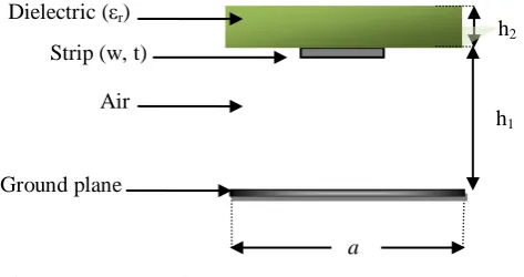
Figure 1 shows the cross section of the shielded inverted microstrip line (IML). The electrical properties of lossless IML lines can be described in terms of the characteristic impedance (Zc), the effective dielectric constant (εeff) and the primary (L and C) parameters [7].
Fig. 1 Cross section of the shielded inverted microstrip line.
Various numerical techniques can be used to determine the electromagnetic parameters (EM) of the IML line [4], [8]. However, they are too time-consuming for direct use in circuit design.
Closed-form analytical models are highly desirable in circuit design [9-11]. This article presents analytical expressions for the EM parameters (Zc, εeff, L and C) of the IML line, deduced from analysis results of the structure by the finite element method (FEM) under freeFEM environment [12], and curve fitting techniques.
h
1Strip (w, t)
Dielectric (ε
r)
Ground plane
a
h
2II.
FEM
RESULTS
In order to find the EM parameters of the IML line, we were interested in the analysis of the structure presented in figure 1 having a dielectric material of εr=2.22. We applied the FEM-based numerical tool to the analysis of the IML line with FEM meshes of the structure shown in figure 2.
Fig. 2 FEM meshes of the IML line.
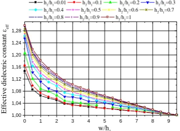
For different (w/h1) and (h2/h1) ratios varying respectively between 0.01-9.5 and 0.01-1, the obtained results by the finite element method (FEM) are shown in figures 3 to 6.
0 1 2 3 4 5 6 7 8 9 10 50
75 100 125 150 175 200 225
h2/h1=0.01 h2/h1=0.1 h2/h1=0.2 h2/h1=0.3
h2/h1=0.4 h2/h1=0.5 h2/h1=0.6 h2/h1=0.7
h2/h1=0.8 h2/h1=0.9 h2/h1=1
w/h1
Ch
ar
ac
ter
istic imp
ed
an
ce
Z
c
(
)
Fig. 3 Characteristic impedance of the IML as a function of w/h1 for various values of h2/h1.
0 1 2 3 4 5 6 7 8 9 1,00
1,04 1,08 1,12 1,16 1,20 1,24 1,28
h2/h1=0.01 h2/h1=0.1 h2/h1=0.2 h2/h1=0.3
h2/h1=0.4 h2/h1=0.5 h2/h1=0.6 h2/h1=0.7
h2/h1=0.8 h2/h1=0.9 h2/h1=1
Effe
ct
ive
di
el
ect
ric
c
ons
ta
nt
eff
w/h1
0 1 2 3 4 5 6 7 8 9 10 100
200 300 400 500 600 700 800
h2/h1=0.01 h2/h1=0.1 h2/h1=0.2 h2/h1=0.3
h2/h1=0.4 h2/h1=0.5 h2/h1=0.6 h2/h1=0.7
h2/h1=0.8 h2/h1=0.9 h2/h1=1
w/h1
In
du
ctan
ce
L (nH
/m )
Fig. 5Inductance of the IML as a function of w/h1 for various values of h2/h1.
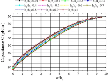
0 1 2 3 4 5 6 7 8 9 10 20
30 40 50 60 70 80 90
h2/h1=0.01 h2/h1=0.1 h2/h1=0.2 h2/h1=0.3
h2/h1=0.4 h2/h1=0.5 h2/h1=0.6 h2/h1=0.7
h
2/h1=0.8 h2/h1=0.9 h2/h1=1
w/h1
Cap
ac
ita
nc
e C (p
F/m
)
Fig. 6 Capacitance of the IML as a function of w/h1 for various values of h2/h1.
The obtained results show that the curves of figures 3 to 6 permit the design of IML lines at characteristic impedances varying between 35 and 225 Ω.
III.
DERIVATION
OF
ANALYTICAL
EXPRESSIONS
A.
Characteristic impedanceUsing curve-fitting, it is found that the characteristic impedance of the IML can be expressed by:
1 /22 / 1
t u t
u co
c
Z
A
e
A
e
Z
(1)
Where:
For
0
.
01
r
0
.
5
3
2 12.05
74 . 11 79 . 2 42 .
34 r r r
Zco
3 2
1
83.32
13.47
r
-
478.74
r
905.31
r
A
-r/86.326 2
-1769.1
1882.49
e
A
-r/0.165
1
0.4
-
0.0125e
t
-r/0.071
2
2.7
-
0.026
e
t
1 2
1
;
/
/
h
r
h
h
w
u
For
0
.
5
r
1
0.5)/0.15 --(r
e
0.33
-34.73
co
Z
0.5)/0.3 --(r 1
69.91
0.57
e
A
0.5)/19.7 --(r
e
166.71
-64.02
0.5)/0.06 --(r 2
2.65658
0.04347e
t
1 2
1
;
/
/
h
r
h
h
w
u
B.
Effective dielectric constantThe effective dielectric constant can be given by the equation (2):
2 1 / 2 1 t u t u effo
eff
A
e
A
e
(2) Where:For
0
.
01
r
0
.
6
5 4 3 2
r
212.015
-r
257.11
106.25r
-r
17.1
r
0.974
-0.99
effo
5 4 3 2 1r
144.567
r
168.35
-r
65.24
r
9.8
-r
0.717
0.071
A
5 4 3 2 2r
168.06
r
204.36
-r
83.2
r
12.37
-r
0.66
0.0836
A
5 4 3 21
0.382
1.94
r
-
3.0
r
-
47.81
r
182.85
r
-
176.95
r
t
5 4 3 2 2r
21858.7
r
26237.13
-r
10728.63
r
1727.58
-r
100.0
5.58
t
1 21
;
/
/
h
r
h
h
w
u
For
0
.
6
r
1
0.6)/0.007 --(r
e
0.035
-0.91
effo
r
0.052
-0.168
1
A
4 3 22
8.56
-
41.4
r
76.6
r
-
62.37
r
18.92
r
A
4 3
2
1
52
-
263.92
r
506.085
r
-
429.12
r
135.65
r
t
4 3 2 2r
2621.25
r
8615.93
-r
10561.91
r
5725.83
-1167.9
t
1 21
;
/
/
h
r
h
h
w
u
C.
Inductance per unit lengthThe inductance of the IML line in (nH/m) is given by relation (3). 2.6
/ 0.364
/
412.57768
352.98
115.563
e
ue
uL
(3)Where:
u
w
/
h
1D.
Capacitance per unit lengthFinally the capacitance of the IML line can be expressed by relations (4) and (5).
For
0
.
01
u
2
m
pF
e
A
C
C
o u/t11 (4)
Where:
For
0
.
01
r
0
.
6
5 4 3 2 1
r
66
.
44812
r
65159.186
-r
33595.44
r
7129.36
-r
522.56
-47.72
A
5 4 3 2 1r
2524.9
-r
4055.54
r
2278.1
-r
516.43
r
39
-3.0625
t
1 21
;
/
/
h
r
h
h
w
u
For
0
.
6
r
1
4 3 2
r
1098
-r
3640.86
r
4521.63
-r
2491.91
-456.12
oC
4 3 2 1r
799.67
r
2678.78
-r
3364.8
r
1875.8
-354.35
A
3 21
2.58
15
r
-
15.63
r
4.98
r
t
1 2
1
;
/
/
h
r
h
h
w
u
For
2
u
9
.
5
m
pF
u
B
u
B
A
C
1 2 2(5)
For
0
.
01
r
0
.
5
2
r
26.29
r
3.37
-17.23
A
3 21
12.2
-
5.96
r
47.27
r
-
78.4
r
B
3 2
2
-0.48
0.7
r
-
5.37
r
8.31
r
B
1 2
1
;
/
/
h
r
h
h
w
u
For
0
.
5
r
1
3 2
r
12.12
-r
24.62
r
10.0
-21.345
A
4 0.5)/10.52 --(r 1
11.35
0.99
e
B
0.5)/0.22 --(r 2
-0.57
0.036e
B
1 2
1
;
/
/
h
r
h
h
w
u
E.
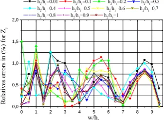
Comparison between analytical and numerical resultsIn figures 7 to 10 we show comparisons between our analytical and numerical results for the IML line.
0 1 2 3 4 5 6 7 8 9 0,0
0,5 1,0 1,5 2,0
h2/h1=0.01 h2/h1=0.1 h2/h1=0.2 h2/h1=0.3
h2/h1=0.4 h2/h1=0.5 h2/h1=0.6 h2/h1=0.7
h2/h1=0.8 h2/h1=0.9 h2/h1=1
w/h1
Relative
s erro
rs in (%) f
or
Zc
0 1 2 3 4 5 6 7 8 9 0,0
0,5 1,0 1,5
h2/h1=0.1 h2/h1=0.2 h2/h1=0.3 h2/h1=0.4
h2/h1=0.5 h2/h1=0.6 h2/h1=0.7 h2/h1=0.8
h2/h1=0.9 h2/h1=1
w/h 1
Relati
ves erro
rs in (%) for
eff
Fig. 8 Relatives errors between analytical and numerical results for the effective dielectric constant of the IML line.
0 1 2 3 4 5 6 7 8 9 0,0
0,5 1,0 1,5 2,0
h2/h1=0.01 h2/h1=0.1 h2/h1=0.2 h2/h1=0.3
h2/h1=0.4 h2/h1=0.5 h2/h1=0.6 h2/h1=0.7
h2/h1=0.8 h2/h1=0.9 h2/h1=1
w/h1
R
elat
ives
errors
i
n (%
) for L
Fig. 9 Relatives errors between analytical and numerical results for the inductance of the IML line.
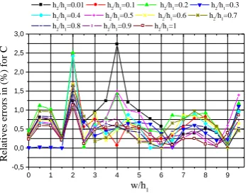
0 1 2 3 4 5 6 7 8 9 -0,5
0,0 0,5 1,0 1,5 2,0 2,5 3,0
h2/h1=0.01 h2/h1=0.1 h2/h1=0.2 h2/h1=0.3
h2/h1=0.4 h2/h1=0.5 h2/h1=0.6 h2/h1=0.7
h2/h1=0.8 h2/h1=0.9 h2/h1=1
w/h1
R
elatives erro
rs in (%) fo
r C
Fig. 10 Relatives errors between analytical and numerical results for the capacitance of the IML line.
From these figures it appears clearly that the relative errors between our analytical and numerical EM-results are less than 2% in a wide range, indicating the good accuracy of the closed-form expressions proposed for the IML line.
IV.
DESIGN
OF
A
3
GHZ
IML
BRANCH
LINE
COUPLER
Fig. 11 Detailed illustration of the IML branch line coupler.
For the IML lines, the dielectric thickness was kept constant. The wide of the strip (w) was varied as needed to change the characteristic impedance of the line. All of the dimensions and the EM parameters, obtained from the proposed analytical expressions, for the coupler lines are provided in table 1.
TABLE I.DESIGNPARAMETERSFORA3GHZBRANCHLINECOUPLERUSINGIMLLINES.
Lines L1 L2
h2/h1 w/h1 Zc (Ω) εeff L (nH/m) C (pF/m) Length (mm)
0.01 9.5 35.5 1. 124.9 99.0 24
0.01 5.0 50.3 1.02 177.7 70.0 24
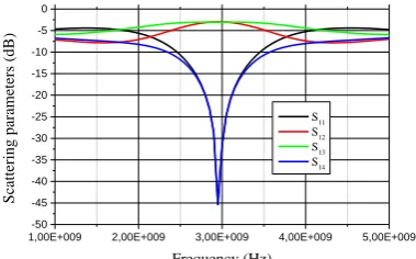
The responses of the designed 3 GHz branch line coupler using IML lines are plotted in figure 12, using an adapted numerical model [13].
1,00E+009 2,00E+009 3,00E+009 4,00E+009 5,00E+009 -50
-45 -40 -35 -30 -25 -20 -15 -10 -5 0
S11
S12
S13
S14
Scatterin
g
pa
ram
eters (d
B)
Frequency (Hz)
Fig. 12 Simulated S-parameters of the IML branch lines coupler.
Figure 12 shows the simulated S-parameters from 1GHz to 5GHz. The simulated insertion loss of the coupler (S13) and direct (S12) paths is better than (-5dB) over the 25% bandwidth from 2.5-3.5GHz. Return loss and isolation are better than (-10dB) over this bandwidth.
V.
CONCLUSION
In summary, the closed-form equations presented here provide simple calculations for the EM parameters of inverted microstrip line (IML) used for microwave and wireless components. These expressions deduced from the finite element method are valid in a wide range of (w/h1) and (h2/h1) ratios varying respectively between 0.01-9.5 and 0.01-1. The formulas were used as the basis for designing an IML branch line coupler operating at 3GHz.
REFERENCES
[1]. R. S. Tomar and P. Bhartia, “New dispersion models for open suspended substrate microstrips,” IEEE MTT-S International Microwave Symposium Digest, pp.387-389, 1988.
[2]. B. E. Spielman, “Dissipation loss effects in isolated and coupled transmission lines, IEEE-Trans. Microwave Theory tech., (MTT-25) , pp. 648-656, 1977.
[3]. T. Kitazawa et al., Planar transmission lines with finitely thick conductors and lossy substrates,” IEEE Int. Microwave Sym. Dig., , pp. 769-772, 1991.
[6]. Y. Bekri, N. Benabdallah, N. Ben Ahmed, F. T. Bendimerad and K. Aliane, “Analysis and design of shielded suspended and inverted microstrip lines for microwave applications,” Computing Science and Technology International Journal, Vol. 2, no. 1,
pp. 33-38, 2012.
[7]. S. Seghier, N. Benabdallah, N. Benahmed, R. Bouhmidi, “Accurate closed formulas for the electromagnetic parameters of squared caxial lines,” Int. J. Electrn. Commun. (AEÜ), Vol. 62, no 5, pp. 395-400, 2008.
[8]. R. Tomar, Y. M. Antar and P. Bhartia, “Computer-aided-design (CAD) of suspended-substrate microstrips: an overview,” International Journal of RF and Microwave Computer-Aided Engineering, Vol. 15, no. 1, pp. 44-55, 2005.
[9]. N. Benahmed, N. Benabdallah, F.T. Bendimerad, B. Benyoucef and S. Seghier, “Accurate closed-form formulas for the electromagnetic parameters of micromachined shielded membrane microstrip line,” in Proc. IEEE Conf. 8th International Multi-Conference on Systems, Signals & Devices, 2011.
[10]. N. Benahmed, N. Benabdallah, R. Bouhmidi, Y. Bekri, S. Seghier and F.T. Bendimerad, Accurate Closed-form Formulas for the Electromagnetic Parameters of 50 Ω Micromachined Microstrip Directional Couplers, Eighth International Multi-Conference on Systems, Signals & Devices, Multi-Conference on Sensors, Circuits & Instrumentation Systems, March 20-23, 2012, Chemnitz, Germany.
[11]. N. Benahmed, Accurate closed-form expressions for the electromagnetic parameters of the shielded split ring line, Int. J. Electrn. Commun. (AEÜ), Vol. 61, pp. 205-208, 2007, www.FreeFEM.org.