Improvement of Committee Machine Performance to Solve Multiple Response Optimization Problems

(1)

Improvement of Committee Machine

Performance to Solve Multiple Response

Optimization Problems

Seyed Jafar Golestaneh*

1

, Napsiah Ismail

2

, Say Hong Tang

3

, Mohd Khairol Anuar M. Ariffin4, Hassan Moslemi

Naeini

5

1,2,3,4_{Department of Mechanical and Manufacturing Engineering, Universiti Putra Malaysia, 43400 Serdang, Selangor,}

Malaysia.

5_{Faculty of Engineering, Tarbiat Modares University, P.O. Box 14155-143 Tehran, Iran} 1_{Industrial Engineering PhD student, Corresponding author, [email protected]}

1_{Mechanical Engineering PhD, [email protected]} 1

Mechanical Engineering PhD, [email protected] 1

Mechanical Engineering PhD, [email protected]

Abstract-- Three phases are considered for multiple response optimization (MRO) problems. They are design of experiments, modeling and optimization. Committee machines (CM) as a set of some experts such as some artificial neural networks (ANNs) can be applied for modeling phase. Then, genetic algorithm (GA) determines the final solution with object maximizing the global desirability as optimization phase. That algorithm was implemented on five MRO case studies include target, minimizing and maximizing objects. Current article is a development of recent authors' work on application of CM in MRO problem solving. Initial approach in that work, includes a committee machine with four different ANNs. The CM weights are specified with GA which its fitness function was minimizing the overall RMS E for each response. In current work, a new approach was applies in finding the committee machine weights. The fitness function in this approach is made by minimizing the absolute error between CM responses and real data for each response, separately. A performance index is defined to evaluate different models performance. The results from five case studies show that there are noticeable decreasing in overall RMS E whereas there is a negligible decreasing in GD for new CM with respect to initial CM. this is due that less error is a confirmation of performance increasing for new committee machine.

Index Term-- Global desirability, Committee Machine, Multiple responses optimization, Genetic Algorithm

I. INT RODUCT ION

Current study is a development in authors recent works [1]. It bodes application of committee machine in modeling of Multiple Response Optimization (MRO) problems. MRO would like to find a set of input variable amounts (x's) which yields a desired set of outputs (y's). MRO as usual is solved in three phases include experiments design, modeling and optimization.

Experiments design is arranged based on some known patterns in Design of Experiments (DOE) knowledge such as factorial design, fraction factorial design. Some deigns in Response Surface Methodology (RSM) such as Central Composite

Design (CCD) and Box Behnken [2, 3]. Also, Taguchi orthogonal arrays [4-7] which is derived from Taguchi method.

Second phase is done by means of different mathematical or statistical modeling such as multiple linear and nonlinear regression in the form of polynomials [2, 8, 9] and Artificial Neural Networks (ANNs). Due to the fact that relationship between inputs and outputs usually are complicated, ANNs mostly are used for modeling rather than polynomials. A typical Artificial Neural Network (ANN) is Back Propagation Neural Network (BPNN) that is used in many engineering problems [10, 11]. Cheng et al. [12] used MANFIS (Multi Adaptive Neuro Fuzzy Inference System) for modeling and showed the results are superior to RSM polynomial models.

Last phase is optimization that usually is done on global desirability function. In this process, every predicted response is converted to a value between 0 to 1 by a function with name desirability function. So for all responses, a composite function is defined which converts all desirability functions to a unique number by global desirability function (GDF). Then with optimization of GDF, optimum or optimal values of independent parameters could be found. Different optimization techniques were used to optimize GDF, for example Excel solver, search methods such as Hook and Jeeves [2], Evolutionary Algorithms such as Genetic algorithm [9, 11] and Tabu Search [10]. Also, Chatsirirungruang and Miyakawa[13] proposed a combination of GA with Taguchi and have used benefits of these techniques together to get more accurate responses.

II. SCOPE AND LIMIT AT IONS

(2)

International Journal of Engineering & Technology IJET-IJENS Vol:13 No:03 53

I J E N S

IJENS © June 2013 IJENS -IJET -9595 -03 1380

"In rang" and this can be a good area to develop this approach in future. This article shows application of committee machine in multiple response optimization can decrease modeling errors and increase reliability of global desirability prediction. on the other hand this work introduce a container which includes different neural networks methods and also traditional modeling method or multiple regression. so due to its capacity to accept newer methods in future, capability of this approach can be increase with progress in time and method.

Artificial neural networks and Committee Machine There are different kinds of neural networks to model and apply in complicated prediction problems. This study has considered four neural networks. They are Feed Forward Neural Networks (FF)[14], Radial Basis function networks (RBFN) [15], Generalized Regression neural network (GRNN)[16] also, Adaptive Neural Fuzzy Inference System (ANFIS) [17, 18].

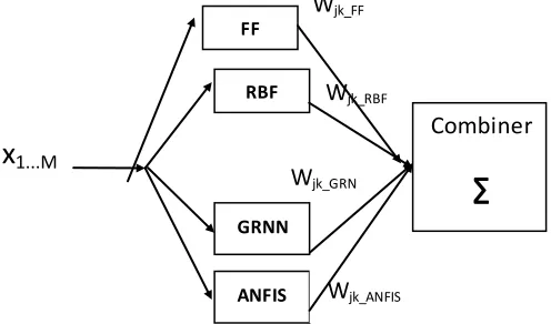
A Committee Machine (CM) consists of a group of intelligent systems named Experts, and a combiner, which combines the outputs of each expert (Figure 1). Its advantages are that it reaps the benefits of all work with only little additional computation. Inputs are entered to experts, and all experts' responses are transferred to a combiner to get final response.

Fig. 1. A typical architecture of a committee machine based on static structure

To combine the experts' outputs, there are different ways in the combiner. It could be an intelligent system such as a neural network. The most popular method is the simple ensemble averaging method according to equation 1[19].

∑

(1)

Where N is the total number of the experts used, wi is the weight coefficient of ith expert and yi is the estimated response from ith expert [20].

Genetic Algorithm could be obtained combination of the experts' contribution (weights) in a committee machine. Equation 2, represents committee machine gives smaller errors than the average of all the experts [20, 21].

o [ ∑ ]≤ ∑ [ ] o (2)

is error of predicted and real response of every ANN or expert. is squared error for the ith expert. o is the average error for each of the experts acting alone. o is error of CM.

Genetic algorithm and global desirability

Genetic Algorithm (GA) can quickly and reliably solve problems that are difficult to tackle by traditional methods. It is extensible and can interface with existing models and hybridize with them and optimizes the fitness function. [22]; [23].

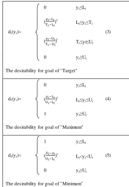
Global desirability Function is used to convert a problem of multiple responses into a single response case. By desirability function, each estimated response is converted into a dimensionless desirability value di. For different situations, di values are defined by the continuous function which are shown in table I [24, 25].

TABLE I

DESIRABILITY FUNCTIONS FORMULA WITH DIFFERENT OBJECTS

di(yi)=

0 yi≤Li

(3) (

)

s

Li≤yi≤Ti

( )

t

Ti≤yi≤Ui

0 yi≥Ui

The desirability for goal of "Target"

di(yi)=

0 yi≤Li

(4) (

)

s

Li≤yi≤Ui

1 yi≥Ui

The desirability for goal of "Maximum"

di(yi)=

1 yi≤Li

(5) (

)

s

Li<yi<Ui

0 yi≥Ui

(3)

The parameters s and t in formulas in table 1 are convexity coefficients and specify how strictly target value will be desired. In current study, both of them are equal to one. Global desirability (GD) is defined as equation 6:

√∏

(6)

Equations of 3 to 5, yields the desirability for different objects and equation 6 calculates the global desirability (GD). The di's range varies from zero to one, and respectively GD rang is from 0 to 1. Important notice is that optimization of GD depends to all desirabilities and thus denoted as simultaneous optimization of all responses.

III. MET HODOLOGY

Dixit and Chandra [26] have suggested a selection method for training data sets for ANNs. They represented for n input, the minimum number of training set should be such that it includes the corners of n-dimensional space with respect to more contribution for input variables with more influence on output. But in current research, this offer was applied for corners of lower and upper limits for all variables. Training to test data numbers was 80-20 percent.

There are different criteria to assess forecasting models performance. In current work two criteria were selected to compare simulated results from models and the observed or real data. They are Root mean square error (RMSE),[27], correlation coefficient (R)[28].

RMSE= √(

𝑁∑ (𝑦𝑖− 𝑦̂𝑖) ) 𝑁

𝑖 (7)

R= ∑𝑁𝑖 =1(𝑦𝑖 𝑦̅𝑖) (𝑦̂𝑖−𝑦̂̅𝑖)

√(∑𝑁_𝑖=1(𝑦_𝑖 𝑦̅_𝑖)2_(𝑦̂_𝑖−_𝑦̂̅_𝑖)2) -1≤R≤+1

(8)

̂ s ith predicted value (model output), is the ith actual value, and n is the number of data used for prediction. Also ̅ and ̂̅ are the mean of actual and predicted values. [29]. There are two conditions to build ANNs model in the current work. The first condition is that RMSE for all data be minimum. The Second condition is that correlation coefficient of testing data is positive.

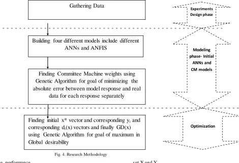
As it is mentioned, MRO solution includes three phases. First, Design of Experiments phase which in the current work, all data is selected from literatures. Second, modeling which is done by building four different neural networks include feed forward, RBF, GRNN and one ANFIS models. All ANNs have same inputs and one output and so the number of ANNs in every model is equal to the number of responses (Figure 2) [1].

Fig. 2. Input and Outputs of every model

A committee machine (CM) was established by combination of all four models (Figure 3). M Inputs are entered to every expert of CM simultaneously, and N responses are multiplied to their weights and then are added together to get final response. CM combiner is an ensemble averaging. CM weights were determined by Genetic Algorithm (GA) with the object to minimize absolute error between real data and CM response foe each response separately. So the total number of weights is 4 multiply by No. of ys (N) multip ly by No. of experiments (r).

Fig. 3. Committee Machine architecture

Current article is a development of recent authors' work on application of CM in MRO problem solving. Initial approach in that work, includes a committee machine with four different ANNs. The CM weights are specified with GA which its fitness function is minimizing the overall RMSE for each response. Then, another GA determines the final solution with object maximizing the global desirability.

According to current algorithm, firstly, all ANNs are created separately to solve the MRO problem. In the modeling phase, first committee machine (CM) weights are calculated by means of GA with the object of minimizing absolute error between real responses and CM responses for each response, separately. Then as optimization phase, GA gets best responses with the object of maximizing global desirability.

y

j

j=1...N

X

1

X

2

X

M

ANN

1...N

y

jk

W

jk_GRN

N

W

jk_FF

W

jk_RBF RBF

FF

Combiner

∑

x

_1...M

GRNN

ANFIS

W

jk_ANFIS

(4)

I J E N S

IJENS © June 2013 IJENS

-IJET -9595 -03 1380

To evaluate performance of all models include ANNs and CMs, a model performance index (P index) is defined as formula 9. Then for all models, the P index is calculated.

Figure 4 shows schematic of proposed methodology, also pseudocode is as follow:

get Data //include X,Y matrixes

setRMSE_network =1 // beginning of modeling phase

set min_RMSE=0.4

for all kind of neural networks

while (RMSE_network>min_RMSE or coefficient of correlation<0)

set X and Y

if min_RMSE> RMSE_network set min_RMSE=RMSE_network end if

add one to iterations

end // end of while

end for

calculate CM weights using GA randomly train network

calculate RMSE_network and coefficient of correlation if RMSE_network<min_RMSE for goal of minimizing in overall RMSE

calculate CM weights by GA with object minimizing absolute error between y CM and y real for each response separately.

// end of modeling phase calculate X*1, y*1 and GD(X*1 )using GA for goal of maximizing in Global desirability //

IV. RESULT S AND DISCUSSION

Genetic algorithm is used for finding CM weights with object of object minimizing absolute error between y CM and y real for each response separately. Also GA was used to find final responses with maximum global desirability.

For all of them, GA specifications are as table 2. P fo manc In x_mod

mod max ( _s) m n (RMS _s)

RMS mod

(9)

Fig. 4. Research Methodology

Finding initial x* vector and corresponding y

i

and

corresponding d

i

(x) vectors and finally GD(x)

using Genetic Algorithm for goal of maximum in

Global desirability

Finding Committee Machine weights using

Genetic Algorithm for goal of minimizing the

absolute error between model response and real

data for each response separately

Building four different models include different

ANNs and ANFIS

Gathering Data

Experiments Design phase

Modeling phase- Initial

ANNs and CM models

(5)

TABLE II GASP ECIFICATION

Variable Magnitude/Kind Variable Magnitude/Kind

Parent population 20 Mutation type Uniform

Selection Function Stochastic Uniform Number of variables 5

Number of elites 2 Number of responses 1

Crossover Fraction 0.8 Migration Direction 'forward'

Crossover Function Scattered Migration Fraction 0.2

Five MRO problems were selected to solve with CM. These problems contain different number of inputs and outputs, also

different number of experiments. Their properties are shown in table 3.

TABLE III CASES P ROP ERTIES

Case No.

No. of x's (m)

No. of y's (N)

No. of

Experiments (r) Reference Objects

1 3 6 15 (Noorossana et al., 2008) T T T T T

T

2 4 2 18 (Giordano et al., 2010) nX

3 3 3 30 (Martinez Delfa et al., 2009) T T T

4 2 2 13 (Bhatti et al., 2011) Xn

5 4 4 30 (Aggarwala et al., 2008) nXnn

T:Target X:Maximu m n:Minimum

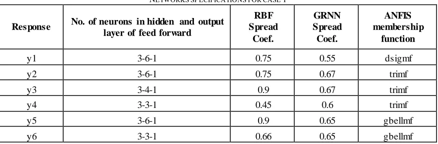
Case1: The problem is based on the wire-bonding process in the semiconductor industry. The process inputs and outputs have shown in table 4. Different neural networks were made to model data of experiments. These ANNs specifications are listed in table 5. To have better comparison between committee machine and other neural networks, same specifications were considered for all other cases as table VI except case 3, and that was due to get acceptable results. Four

ANNs include feedforward (FF), Radial Base Function (RBF), GRNN and ANFIS were consisted for every response for every problem data. So every problem has found (4*No of responses) models. Consequently, the results of other models are listed in table 6. A committee machine was made with object minimizing absolute error between y CM and y real for each response separately.

TABLE IV

INP UT AND RESP ONSE VARIABLES AND OP TIMIZATION CRITERIA FOR EVERY RESP ONSE (OUTP UT) IN CASE 1

Input (Independent) Variables Output(De pendent) Variables Opt. criteria

x1: Flow rate (SCFM) y1: Maximum temperature at position A (°C) Target

x2: Flow temp (°C) y2: Beginning bond temperature at position A (°C) Target

x3: Block temp (°C) y3: Finish bond temperature at position A (°C) Target

y4: Maximum temperature at position B (°C) Target

y5: Beginning bond temperature at position B (°C) Target

(6)

I J E N S

-IJET -9595 -03 1380

TABLE V

NETWORKS SP ECIFICATIONS FOR CASE 1

Response No. of neurons in hidden and output layer of feed forward

RBF Spread

Coef.

GRNN Spread Coef.

ANFIS membership

function

y1 3-6-1 0.75 0.55 dsigmf

y2 3-6-1 0.75 0.67 trimf

y3 3-4-1 0.9 0.67 trimf

y4 3-3-1 0.45 0.6 trimf

y5 3-6-1 0.9 0.65 gbellmf

y6 3-3-1 0.66 0.65 gbellmf

Case2: The problem is to optimize the yield of recombinant Oryza sativa non-symbiotic hemoglobin 1 in medium

containing byproduct glycerol. The input and output variables have listed in table 7.

TABLE IV

NETWORKS SP ECIFICATIONS FOR CASES 2-5 FOR ALL Y'S

Case No. No. of neurons in hidden and output layer of feed forward

RBF Spread Coef.

GRNN Spread Coef.

ANFIS membership

function

2,4,5,6 3-1 0.85 0.5 gbellmf

3 3-5-1 0.85 0.45 gbellmf

TABLE VII

INP UT AND RESP ONSE VARIABLES AND OP TIMIZATION CRITERIA FOR EVERY RESP ONSE (OUTP UT)(CASE 2)

x1: Tryptone. (g L−1) y1: Biomass. (g L −1

) Minimize

x2: Yeast extract (g L−1)

y2: Oryza sativa non-symbiotic

hemoglobin1_ OsHb1 (g L−1) Maximize x3: Sodium chloride (g L−1)

x4: Byproduct glycerol (g L−1)

Case3: the problem is multiple response optimization of styrene–butadiene rubber (SBR) emulsion batch

polymerization. The input and output variables have listed in table VIII.

TABLE VIII

Initiator (mL) solid content of latex (wt%) Target

Activator (mL) Mooney viscosity Target

Chain transfer agent_CTA (mL) polydispersity Target

Case 4: Object of this case is to optimize process variables, electrolysis voltage and treatment time for the electro

(7)

TABLE IX

x1: Voltage(V) y1: Reduction efficiency (%) Maximize

x2: Time(min) y2: Energy consumption (Wh) Minimize

Case 5: problem is to optimize multiple characteristics in CNC turning of AISI P-20 tool steel using liquid nitrogen as a coolant. The input and output variables have listed in table 10.

TABLE X

Cutting speed (m/min) Surface roughness (_m) Minimize

Feed (mm/rev) Tool life (min) Maximize

Depth of cut (mm) Cutting force (N) Minimize

Nose radius (mm) Power consumption (W) Minimize

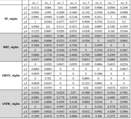
Table XI represents weigths of committee machine in initial approach for case 1 and tables XII ans XIII represent these

weights in new approach. As mentioned total number of weights is 36 (4*6*15).

TABLE XII

COMMITTEE MACHINES WEIGHTS BY GA IN NEW AP P ROACH (CASE 1_EXP ERIMENTS 1-8)

no_1 no_2 no_3 no_4 no_5 no_6 no_7 no_8

FF_wights

y1 0.1111 0.006 0.01 0.0695 0.3205 0.9886 0.0504 0.2369

y2 0.9995 0.999 0.2889 0.1605 0.1192 0.5556 0.1044 0.9908

y3 0.0001 0.9969 0.1605 0.2148 0.9998 0.3611 1 0.001

y4 1 0.0364 0.2577 0.0777 0.9999 0.3792 0.1111 0.2

y5 0.9962 0.8 0.1111 0.1671 0.102 0.0007 0.1583 0.1993

y6 0.1252 0.0067 0.0285 0.0701 0.0109 0.0383 0.168 0.9346

RBF_wights

y1 0.4444 0.8954 0.286 0.0011 0.3432 0.0017 0.1522 0.0315

y2 0.0001 0.0006 0.5333 0.3457 0.4394 0 0.4273 0.0001

y3 0.7604 0.0018 0.3457 0.3704 0 0.4509 0 0

y4 0 0.2206 0.3426 0.7929 0 0.3104 0.3111 0.2667

y5 0.0006 0.1728 0.4446 0.4066 0.7505 0.0009 0.4209 0.5101

y6 0.4417 0.0096 0.1742 0.0313 0.0013 0.633 0.6069 0.0101

GRNN_wights

y1 0 0.0203 0.0815 0.0595 0.1495 0.0084 0.6033 0.0236

y2 0.0003 0.0001 0 0 0 0 0 0.0017

y3 0.0829 0.0007 0 0 0 0.1686 0 0

y4 0 0.702 0 0 0.0001 0 0 0

y5 0.0028 0.0247 0 0 0.1323 0.0002 0 0

y6 0.2123 0.0359 0 0 0.02 0.0207 0.0276 0.0315

ANFIS_wights

y1 0.4444 0.0783 0.6224 0.87 0.1868 0.0013 0.1941 0.7081

y2 0.0001 0.0003 0.1778 0.4938 0.4414 0.4444 0.4683 0.0075

y3 0.1567 0.0006 0.4938 0.4148 0.0002 0.0194 0 0.9989

y4 0 0.0411 0.3997 0.1293 0 0.3104 0.5778 0.5333

y5 0.0004 0.0026 0.4443 0.4263 0.0152 0.9982 0.4209 0.2906

(8)

I J E N S

-IJET -9595 -03 1380

TABLE XI

COMMITTEE MACHINES WEIGHTS BY GA IN INITIAL AP P ROACH (CASE 1)

Model y1 y2 y3 y4 y5 y6

FF 0.0121 1.0000 0.0768 0.0019 0.4402 0.1567

RBF 0.5377 0.0000 0.3966 0.2612 0.0145 0.0400

GRNN 0.0405 0.0000 0.0000 0.0034 0.0007 0.1210

ANFIS 0.4097 0.0000 0.5266 0.7335 0.5447 0.6823

TABLE XIII

COMMITTEE MACHINES WEIGHTS BY GA IN CURRENT AP P ROACH (CASE 1_EXP ERIMENTS 9-15)

no_9 no_10 no_11 no_12 no_13 no_14 no_15

FF_weights

y1 0 0.4866 0.032 0.017 0.0198 0.7359 0

y2 0.0017 0 0.9235 0.0306 0.0071 0.2 0.0002

y3 0.1101 0.993 0.1111 0.4403 0.1322 0.0215 0.1111

y4 0.1131 0.2 0.9989 0.52 0.0156 0.0001 0.9999

y5 0.2527 0.0112 0.9772 0.1605 0.0004 0.1383 0.0047

y6 0.1111 1 0.0713 0.0065 0 1 0.4269

RBF_weights

y1 0.8526 0.333 0.9094 0.4227 0.9098 0.2205 0.3379

y2 0.7811 0.91 0.0093 0.2242 0.0355 0.5333 0.1529

y3 0.4447 0.0019 0.4444 0.0025 0.8094 0.0771 0.4444

y4 0.111 0.2667 0.0004 0.2391 0.0904 0.1558 0

y5 0.0557 0.6089 0.0165 0.3456 0.1245 0.7915 0.1727

y6 0.8889 0 0.143 0.0501 0.0744 0 0.2753

GRNN_weights

y1 0.0377 0.1584 0 0.0452 0.0704 0.0377 0.6524

y2 0.0034 0.0224 0.0383 0 0.8781 0 0.8279

y3 0.0002 0.0042 0 0.0753 0 0.8387 0

y4 0.3388 0 0.0001 0 0 0.6819 0

y5 0 0.1671 0.0059 0.0001 0.735 0 0

y6 0 0 0.2133 0 0.1226 0 0.2631

ANFIS_weights

y1 0.1098 0.022 0.0585 0.5151 0 0.0058 0.0097

y2 0.2138 0.0676 0.0289 0.7452 0.0792 0.2667 0.019

y3 0.445 0.0008 0.4444 0.482 0.0585 0.0628 0.4444

y4 0.4371 0.5333 0.0006 0.2408 0.894 0.1622 0

y5 0.6916 0.2128 0.0004 0.4938 0.1401 0.0702 0.8226

(9)

TABLE IX

COMP ARISON RESULTS OF OVERALL RMSE,GD AND P ERFORMANCE INDEX OF ALL MODELS (CASE1)

Model RMSE Rmin/R

% change in RMSE

to CM_i

GD G/Gmax

% change in GD to

CM_i

P Index

CM_new 1.90 1.26 -9.6% 0.639 1.03 34.9% 2.29

CM_0 2.10 1.14 0.0% 0.474 0.76 0.0% 1.90

ANNs

Avg 2.65 0.90 26.3% 0.297 0.48 -37.3% 1.38

FF 2.55 0.94 21.4% 0.566 0.91 19.6% 1.85

RBF 2.47 0.97 17.7% 0.000 0.00 -100.0% 0.97

GRNN 3.20 0.75 52.2% 0.000 0.00 -100.0% 0.75

ANFIS 2.39 1.00 13.7% 0.621 1.00 31.1% 2.00

The case 1 is a famous problem in the literature and several researchers investigated different solutions. The premier author of this case was Del Castillo et al. [2]. His approach got the global desirability of 0.306. Another researcher was Ortiz et al. [11]. According to His solution methodology for this problem, the global desirability was 0.408. the third researcher was Nooroassana et al. [11]. He solved this problem with neural network approach. His methodology got GD=0.417. Finally He et al. [30]as last researcher presented GAPS method. It is a hybrid algorithm include coupling of the genetic algorithm (GA) with the pattern search (PS). According to it, the global desirability is equal to 0.363. Table 15 is a comparison of different method to solve problem case 1 and due to the lack of RMSE or MSE for all solutions, just the global desirability is compared. Remark that, current approach tends to show effect of CM with respect to its experts according to table XIV ns superior comparision will happen when both RMSE and GD be available.

TABLE XV

COMPARISON OF DIFFERENT SOLUT IONS FOR CASE 1

Approach GD

Del Castillo et al.[2] 0.306

Ortiz et al.[11] 0.408

Noorossana et al.[11] 0.417

HE et al.[30] 0.363

Golestaneh et al. [1] 0.474

Current approach 0.639

For abstract, the weights for other cases have not showed. The results of overall RMSE and global desirability for each case are listed in tables 16 to 19. In these tables minimum overall RMSE and maximum GD are derived from best ANNs. So there is a comparison between any model include ANNs or CMs with best expert

Furthermore, another comparison in these tables are between all models and initial committee machines with respect of change percent in overall RMSE and GD.

It can be seen in all cases overall RMSE decreases and as usual GD has decreasing too. But decreasing percent of RMSE is many more than GD.

As a consequence, It can be seen that all new CMs have superior performance index than all ANNs and initial CM .

TABLE XVI

Model RMS E Rmin/R

% change in RMS E to CM_i

GD G/Gmax

% change in GD to CM_i

P Index

CM_new 0.07 6.72 -76.1% 0.720 0.77 -1.1% 7.49

CM_0 0.29 1.61 0.0% 0.727 0.78 0.0% 2.39

ANNs

Avg 0.54 0.86 86.1% 0.747 0.80 2.7% 1.66

FF 0.67 0.70 128.2% 0.933 1.00 28.3% 1.70

RBF 0.47 1.00 60.7% 0.694 0.74 -4.5% 1.74

GRNN 0.56 0.85 89.9% 0.586 0.63 -19.4% 1.47

(10)

I J E N S

-IJET -9595 -03 1380

TABLE XVII

% change in RMSE to CM_i

GD G/Gmax

P Index

CM_new 0.98 5.62 -74.2% 0.969 0.97 -1.6% 6.60

CM_0 3.81 1.45 0.0% 0.985 0.99 0.0% 2.44

ANNs

Avg 9.53 0.58 150.2% 0.978 0.98 -0.7% 1.56

FF 10.54 0.53 176.7% 0.985 0.99 0.1% 1.51

RBF 5.54 1.00 45.3% 0.998 1.00 1.3% 2.00

GRNN 14.70 0.38 285.9% 0.933 0.93 -5.3% 1.31

ANFIS 7.34 0.75 92.8% 0.995 1.00 1.1% 1.75

TABLE XVIII

% change in RMSE to CM_i

GD G/Gmax

P Index

CM_new 0.35 1.30 -22.2% 0.854 0.97 -4.2% 2.28

CM_0 0.45 1.01 0.0% 0.891 1.02 0.0% 2.03

ANNs

Avg 1.16 0.39 158.8% 0.854 0.98 -4.1% 1.37

FF 0.46 0.99 2.2% 0.876 1.00 -1.8% 1.99

RBF 0.45 1.00 1.5% 0.853 0.97 -4.3% 1.97

GRNN 2.38 0.19 431.6% 0.828 0.95 -7.1% 1.14

ANFIS 1.34 0.34 199.8% 0.861 0.98 -3.4% 1.32

TABLE XIX

% change in RMSE to

CM_i

GD G/Gmax

% change in GD to

CM_i

P Index

CM_new 2.00 1.97 -54.3% 0.892 0.98 -1.3% 2.95

CM_0 4.38 0.90 0.0% 0.904 1.00 0.0% 1.89

ANNs

Avg 9.23 0.43 110.9% 0.905 1.00 0.1% 1.42

FF 6.19 0.63 41.6% 0.908 1.00 0.5% 1.63

RBF 13.26 0.30 203.1% 0.904 1.00 0.1% 1.29

GRNN 13.53 0.29 209.1% 0.901 0.99 -0.3% 1.28

ANFIS 3.93 1.00 -10.2% 0.907 1.00 0.4% 2.00

(11)

TABLE XX

GRAP HICAL COMP ARISON OF DIFFERENT MODELS P ERFORMANCE FOR ALL FIVE CASES

A

CKNOWLEDGEM ENT

The authors wish to thank Sadid Industrial Group and especially Eng. A.A. Maghsoudi, for support.

C

ONCLUSION

Different artificial neural networks (ANNs) are used for modeling of multiple response optimization (MRO) problems.

Committee machine is a collection of several elements or experts such as ANNs. Current study is a development of recent authors work on application of committee machine to solve MRO problem. In current new approach, all weights of CM are calculated by genetic algorithm that its fitness function is minimizing absolute error between CM response and real data for each respons. This new approach yields

0.00 0.50 1.00 1.50 2.00 2.50

Performance

Index_case 1

0.00 2.00 4.00 6.00 8.00

Performance

Index_case 2

0.00 2.00 4.00 6.00 8.00

Performance

Index_case 3

0.00 0.50 1.00 1.50 2.00 2.50

Performance

Index_case4

0.00 0.50 1.00 1.50 2.00 2.50 3.00 3.50

(12)

I J E N S

noticeable decreasing in overall RMSE of new CM with respect to initial CM. also there is a negligible decreasing in global desirability. But due to higher accuracy of new CM, its performance is superior than previous one. The results of five case studies include target, minimizing and maximizing objects, represent the improvement in committee machine performance with new approach. Current study represents a classic approach of CM to solve MRO furthermore new approach, which causes development in performance of modeling. In this study, all experts was utilized together, and as a future work it can be investigate the priority for each expert. In addition, combination of experts is a good subject to develop this approach. Another area to development of current work is investigation about possibility of overfitting in modeling by committee machines.

R

EFERENCES

[1] Golestaneh, S.J., et al., A committee machine

approach to multiple response optimization.

International Journal of the Physical Sciences, 2011. 6(35): p. 7935 - 7949.

[2] Del Castillo, E., D.C. Montgomery, and D.R. Mccarviille, Modified desirability function for

multiple response optimization. Journal of quality

technology, 1996. 28(3): p. 337-345.

[3] Guo, W.-l., et al., Optimization of fermentation medium for nisin production from Lactococcus lactis subsp. lactis using response surface methodology (RSM) combined with artificial neural network

-genetic algorithm (ANN-GA). African Journal of

Biotechnology, 2010. 9(38): p. 6264-6272.

[4] Antony, J., et al., Multiple response optimization using Taguchi methodology and neuro -fuzzy based

model. Journal of Manufacturing Technology

Management, 2006. 17(7): p. 908-925.

[5] Chang, H.H., A data mining approach to dynamic multiple responses in Taguchi experimental design. Expert Systems with Applications, 2008. 35: p. 1095–1103.

[6] Kumanan, S., J.E.R. Dhas, and K. Gowthaman, Determination of submergrd arc welding process parameters using taguchi method and regression

analysis. Indian Journal of Engineering & Materials

Sciences, 2007. 12: p. 177-183.

[7] Yao, A.W.L., H.T. Liao, and C.Y. Liu, A Taguchi and Neural Network Based Electric Load Demand

Forecaster. The Open Automation and Control

System Journal, 2008. 1: p. 7-13.

[8] Lepadatu, D., et al., Lifetime Multiple Response

Optimization of Metal Extrusion Die. RAMS 2005

IEEE, 2005.

[9] Pasandideh, S.H.R. and S.T.A. Niaki, Multi-response simulation optimization using genetic algorithm

within desirability function framework . Applied

Mathematics and Computation, 2006. 175: p. 366– 382.

[10] Mukherjee, I. and P.K. Ray, A modified tabu search strategy for multiple-response grinding process

optimisation. International Journal of Intelligent

Systems Technologies and Applications, 2008. 4(1/2): p. 97-122.

[11] Noorossana, R., S.D. Tajbakhsh, and A. Saghaei, An artificial neural network approach to

multiple-response optimization. International Journal of

Advanced Manufacturing Technology, 2008: p. doi: 10.1007/s00170-008-1423-7.

[12] Cheng, C.B., C.-J. Cheng, and E.S. Lee, Neuro-Fuzzy and Genetic Algorithm in Multiple Response

Optimization. Computers and Mathematics with

Applications, 2002. 44: p. 1503-1514.

[13] Chatsirirungruang, P. and M. Miyakawa, Application of genetic algorithm to numerical experiment in robust parameter design for signal multi-response

problem. International Journal of Management

Science and Engineering Management, 2009. 4(1): p. 49-59.

[14] Kamo, T. and C. Dagli, Hybrid approach to the

Japanese candlestick method for financial

forecasting. Expert Systems with Applications, 2009.

36: p. 5023-5030.

[15] Celikoglu, H.B., Application of radial basis function and generalized regression neural network s in non -linear utility function specification for travel mode

choice modelling. Mathematical and Computer

Modelling, 2006. 44: p. 640–658.

[16] Matlab User’s Guide, Version 2010b. Neural Network Toolbox. Math Works,USA, 2010.

[17] Ardil, E. and P.S. Sandhu, A soft computing approach for modeling of severity of faults in

software systems. International Journal of Physical

Sciences, 2010. 5(2): p. 074-085.

[18] Bo, J., T. Yuchun, and Z. Yan-Qing Hybrid SVM-ANFIS for protein subcellular location prediction. International Journal of Computational Intelligence in Bioinformatics and Systems Biology, 2009. 1(1): p. 59.

[19] Ismail, N., et al., Modified committee neural

network s for prediction of machine failure times, in

The 3rd national intelligent systems and information

technology symposium (ISITS 2010). 2010: Institute

of Advanced Technology (ITMA), Universiti Putra Malaysia (UPM)-Malaysia.

[20] Kadkhodaie-Ilkhchi, A., M.R. Rezaee, and H. Rahimpour-Bonab, A committee neural network for prediction of normalized oil content from well log data: An example from South Pars Gas Field,

Persian Gulf. Journal of Petroleum Science and

Engineering 2009. 65: p. 23-32.

(13)

(SCMNN). Journal of Petroleum Science and Engineering, 2010. 73: p. 227–232.

[22] Liang, Y., Combining neural network s and genetic algorithms for predicting the reliability of repairable

systems. International Journal of Quality &

Reliability Management, 2008. 25(2): p. 201-210. [23] Tian, L. and A. Noore, Evolutionary neural network

modeling for software cumulative failure time

prediction. Reliability Engineering & System Safety,

2005. 87: p. 45-51.

[24] Benyounis, K.Y., A.G. Olabi, and M.S.J. Hashmi, Multi-response optimization of CO2 laser-welding

process of austenitic stainless steel. Optics & Laser

Technology, 2008. 40: p. 76-87.

[25] Chang, H.-H. and Y.-K. Chen, Neuro-genetic approach to optimize parameter design of dynamic

multiresponse experiments. Applied Soft Computing,

2011. 11: p. 436–442.

[26] Dixit, U.S. and S. Chandra, A neural network based methodology for the prediction of roll force and roll torque in fuzzy form for cold flat rolling process. International Journal of Advanced Manufacturing Technology, 2003. 22: p. 883–889.

[27] Haghizadeh, A., l. Teang shui, and E. Goudarzi, Estimation of Yield Sediment Using Artificial Neural

Network at Basin Scale. Australian Journal of Basic

and Applied Sciences, 2010. 4(7): p. 1668-1675. [28] Krause, P., D.P. Boyle, and F. B¨ase, Comparison of

different efficiency criteria for hydrological model

assessment. Advances in Geosciences, 2005. 5: p.

89–97.

[29] Banik, S., M. Anwer, and A.F.M. Khodadad Khan, Predictive Power of the Daily Bangladeshi Exchange Rate Series based on Mark ov Model, Neuro Fuzzy

Model and Conditional Heterosk edastic Model, in

12th International Conference on Computer and

Information Technology (ICCIT 2009). 2009: Dhaka,

Bangladesh. p. 303-308.

[30] He, Z. and P.F. Zhu, A hybrid genetic algorithm for

multiresponse parameter optimization within

desirability function framewor, in 16th international

conference of Industrial engineering and engineering