Estimate the Heavy Metal Contamination in Soils Using Numerical Method and Its Application in Iraq

Estimate the Heavy Metal Contamination in Soils

Using Numerical Method and Its Application in Iraq

Luma Naji Mohammed Tawfiq

_{& Israa Najm Abood}

College of Education for Pure Science Ibn Al-Haitham, Baghdad University. * Author to whom correspondence should be addressed; Email: [email protected]

** [email protected]

Abstract-- In this paper a new approach to numerical method based on the theory of interpolation for functions with two variables is proposed. We develop a multivariate divided difference method. In addition, the explicit formulae that connect the classical finite difference interpolation coefficients for one variable curve with multivariate interpolation coefficients are established.

Then to illustrate the accuracy and efficiency of suggested method we used it to estimate the rate of contaminated soils by heavy metals that is evaluate the concentration of heavy metals in soil in Iraq.

Index Term-- Interpolation method, divided difference method, Soil, Heavy metals, Contamination.

Mathematics Subject Classification (2010): 41A05, 65M06, 65D05, 41A63, 78M20, 65Z05,

1. INTRODUCTION

Interpolation theory for functions of one variable has a long and distinguished history, dating back to Newton's interpolation formula and the classical calculus of finite differences, [1-3]. Standard numerical approximations to derivatives and many numerical integration methods for differential equations are based on the finite difference

calculus. However, historically, no comparable calculus was developed for functions of more than one variable. In this paper the extension of divided difference formula for multi variable are introduced with its modification to increase the accuracy and smoothening of method then applied the suggested formula to estimate the contamination in soils by heavy metals.

Heavy metals in the soil refers to some significant heavy metals of biological toxicity, including zinc (Zn), copper (Cu), nickel (Ni), cadmium (Cd), lead (Pb), chromium (Cr), and arsenic (As), etc. With the development of the global economy, both type and content of heavy metals in the soil caused by human activities have gradually increased in recent years, which have resulted in serious environment deterioration. In present study we compared and analyzed suggested method with other to estimate the soil contamination by heavy metals in various zone in Alkhuyls

city appurtenance to Khalis city in Iraq country. In recent years, there are many studies about this problem for its importance such [4-11] but these studies used statistical methods for processing the data. Also, there are many studies which processing the data mathematically such [12-18]. This work consist different method for choosing and processing the data.

2.DIVIDED DIFFERENCE METHOD

Let f(x) be a continuous function given at the distinct point xi, i= 0,1, 2,…,n, define the zeros divided difference of the function f with respect to xi denoted f[xi] by

f[xi] = f(xi), The first divided difference of the function f with respect to xi and xi+1 denoted f[x0 ,x1] and is defined as [19]:

𝑓[𝑥0, 𝑥1] =𝑓[𝑥1

] − 𝑓[𝑥0]

𝑥1− 𝑥0

The second divided difference denoted f[xi, xi+1, xi+2] and is defined as:

𝑓[𝑥0, 𝑥1, 𝑥2] =

𝑓[𝑥1, 𝑥2] − 𝑓[𝑥0, 𝑥1]

𝑥2− 𝑥0

Similarly the nth divided difference relative to x0, x1,…., xn-1, xn, is given by

𝑓[𝑥0, 𝑥1, … . . , 𝑥𝑛−1, 𝑥𝑛] =𝑓[𝑥1,𝑥2,…..,𝑥𝑛_𝑥]−𝑓[𝑥0,𝑥1,….,𝑥𝑛−1]

𝑛−𝑥0 (1)

i.e., if i= 0, 1, 2, then 𝑓[𝑥𝑜, 𝑥1, 𝑥2] = 𝑓[𝑥1, 𝑥0, 𝑥2] = 𝑓[𝑥2, 𝑥1, 𝑥0].

The following theorem describes the relation between nth divided difference formula of the function andits derivative.

Theorem 1 [20]

𝐼𝑓ƒ(𝑛)_{(𝑥) is continuous in [𝑎, 𝑏] and 𝑥}

0, 𝑥1, … , 𝑥𝑛 are in [ a, b] than

ƒ[𝑥0, 𝑥1, … , 𝑥𝑛] =ƒ

(𝑛)_(𝜉)

𝑛! (2)

Where; min (𝑥0, 𝑥1, … 𝑥𝑛) ≤ 𝜉 ≤ max (𝑥0, 𝑥1, … 𝑥𝑛 )

A particular case ofTheorem 1, is the following corollary.

Corollary 1

If ƒ(𝑛) (𝑥) is continuous in a neighborhood of 𝑥 than

ƒ [𝑥, 𝑥, . . , 𝑥⏟

𝑛+1𝑡𝑒𝑟𝑚𝑠

] =ƒ

(𝑛) _(𝑥)

𝑛!

3.MULTI INTERPOLATION METHOD

The problems of polynomial interpolation for functions of several independent variables are important but the methods are less well developed than in the case of functions of a one variable. Causes of the difficulties inherent in the higher dimensional case can be seen in the lack of uniqueness in the general interpolation problem. That is, we ask if x1, x2,… , xm are 𝑚 distinct points,

say in the 𝑥, 𝑦_plane, and then is there a unique polynomial of specified degree which attains specified values, say 𝑓(𝑥1), at these

points? Clearly the answer, in general, must be no since if all of the points (x1, f(x1)) lie on a straight line in 𝑥, 𝑦, 𝑧_space than there are infinitely many planes (i.e., linear polynomials) and perhaps higher degree polynomials of the from 𝑧 =

ℎ(𝑥, 𝑦) containing this line. We shall not dwell on these aspects of interpolation in higher dimensions but shall how to construct appropriate polynomials when the points of interpolation are specially chosen. It will also be found that in these special cases the interpolation polynomials are unique. For simplicity, we concentrate on functions of two variables but extension to more dimensions offers no difficulty.

Another representation of the interpolation polynomial can be obtained by using divided difference formulae, with the 𝑚 + 1 distinct points 𝑥𝑖 we have:

ƒ(𝑥, 𝑦) = ∑𝑚𝑖=0𝑤𝑖−1(𝑥) ƒ[𝑥0 , 𝑥1 ,…,𝑥𝑖 ;𝑦] +𝑤𝑚(𝑥)ƒ[𝑥0,… , 𝑥𝑚, 𝑥; 𝑦 ] (3)

where;

𝜔−1(𝑥) ≡ 1; 𝜔𝑖(𝑥) = 𝜔𝑖−1(𝑥) (𝑥 − 𝑥𝑖), 𝑖 = 0,1, … ;

The divided differences of a function of several variables are formed by keeping all but one variable fixed and taking the

indicated differences with respect to the free variable. Hence ƒ[𝑥0,𝑥1, … , 𝑥𝑖; 𝑦]as a function of the independent variable 𝑦 has the

Newton representation, using the 𝑛 + 1 𝑝𝑜𝑖𝑛𝑡𝑠 𝑜𝑓 𝑦_𝑗:

ƒ[𝐱𝟎, 𝐱𝟏 , … , 𝐱𝐢; 𝐲] = ∑𝐧𝐣=𝟎𝛚𝐣−𝟏(𝐲)ƒ[𝐱𝟎, 𝐱𝟏, … , 𝐱𝐢; 𝐲𝟎,𝐲𝟏, … , 𝐲𝐣]+ 𝛚𝐧(𝐲)ƒ[𝐱𝟎, … , 𝐱𝐢; 𝐲𝟎,… , 𝐲𝐧, 𝐲] (4)

We use equation (4) for 𝑖 = 0 , 1, … , 𝑚 in equation(3)to get

ƒ(𝑥, 𝑦) = 𝑄(𝑥, 𝑦) + 𝑅(𝑥, 𝑦)

𝑄(𝑥, 𝑦) = ∑𝑖=0𝑚 ∑𝑛𝑗=0𝜔𝑖−1 (𝑥) 𝜔𝑗−1 (𝑦)ƒ[𝑥0, … , 𝑥𝑖; 𝑦0, … 𝑦𝑗] (5)

and

𝑹(𝒙, 𝒚) = 𝝎𝒏(𝒚) ∑𝒎𝒊=𝟎𝝎𝒊−𝟏(𝒙)ƒ[𝒙𝟎, … , 𝒙𝒊; 𝒚𝟎, … , 𝒚𝒏, 𝒚]+ 𝝎𝒎(𝒙)ƒ[𝒙𝟎, … , 𝒙𝒎, 𝒙; 𝒚] (6a)

It is clear that 𝑅(𝑥_𝑖 , 𝑦_𝑗) = 0 at the (𝑚 + 1)(𝑛 + 1) points. To simplify this expression we again use Newton's formula and the

𝑚 + 1 𝑝𝑜𝑖𝑛𝑡𝑠 𝑥𝑖 to write

ƒ[𝐱; 𝐲𝟎, … , 𝐲𝐧, 𝐲] = ∑ 𝛚𝐢−𝟏(𝐱)ƒ[𝐱𝟎, … , 𝐱𝐢; 𝐲𝟎, … , 𝐲𝐧, 𝐲] + 𝛚𝐦(𝐱)ƒ[𝐱𝟎, … , 𝐱𝐦, 𝐱; 𝐲𝟎, … , 𝐲𝐧, 𝐲] 𝐦

𝐢=𝟎

If we multiply this identity by 𝜔𝑛(𝑦) and subtract the result from (6a) we obtain finally,

𝐑(𝐱, 𝐲) = 𝛚𝐦(𝐱)ƒ[𝐱𝟎, … , 𝐱𝐦, 𝐱; 𝐲] + 𝛚𝐧(𝐲)ƒ[𝐱; 𝐲𝟎, … , 𝐲𝐧,𝐲] − 𝛚𝐦(𝐱)𝛚𝐧(𝐲)ƒ[𝐱𝟎, … , 𝐱𝐦, 𝐱; 𝐲𝟎, … , 𝐲𝐧, 𝐲](6b)

If ƒ(𝑥, 𝑦) has continuous partial derivatives of orders 𝑚 + 1 𝑎𝑛𝑑 𝑛 + 1, respectively in 𝑥 𝑎𝑛𝑑 𝑦 and the appropriate mixed derivative of order 𝑚 + 𝑛 + 2 then the error becomes

𝑹(𝐱, 𝐲) = 𝛚𝐦 (𝐱)

(𝐦+𝟏)!

𝛛𝐦+𝟏_{ƒ(𝛏,𝐲)}

𝛛𝐱𝐦+𝟏 +

𝛚_𝐧(𝐲)

(𝐧+𝟏)!

𝛛𝐧+𝟏_ƒ(𝐱,ŋ)

𝛛𝐲𝐧+𝟏 −

𝛚_𝐦 (𝐱)𝛚_𝐧(𝐲)

(𝐦+𝟏)!(𝐧+𝟏)!

𝛛𝐦+𝐧+𝟐 ƒ(𝛏′,ŋ′) 𝛛𝐱𝐦+𝟏 _𝛛𝐲𝐧+𝟏 (7) We obtain, upon replacing 𝑚 𝑏𝑦 𝑛 𝑖𝑛 (3) 𝑎𝑛𝑑 𝑛 𝑏𝑦 𝑛 − 𝑖, in (4)

ƒ(𝑥, 𝑦) = 𝑃𝑛(𝑥, 𝑦) + 𝑅𝑎(𝑥, 𝑦)

where

𝑃𝑛(𝑥, 𝑦) = ∑𝑛𝑖=0∑𝑛−𝑖𝑗=0𝜔𝑖−1(𝑥)𝜔𝑗−1(𝑦)𝑓[𝑥0, … , 𝑥𝑖; 𝑦0, … , 𝑦𝑗] (8)

and

𝑅𝑛(𝑥, 𝑦) = ∑𝑛𝑖=0𝜔𝑖−1(𝑥)𝜔𝑛−𝑖(𝑦)𝑓[𝑥0, … , 𝑥𝑖; 𝑦0, … , 𝑦𝑛−𝑖, 𝑦] + 𝜔𝑛(𝑥)𝑓[𝑥0, … , 𝑥; 𝑦]

= ∑ 𝜔𝑖−1(𝑥)𝜔𝑛−𝑖(𝑦)

𝑖!(𝑛−𝑖+1) 𝑛+1

𝑖=0 (_𝜕𝑥𝜕)

𝑖

(_𝜕𝑦𝜕)𝑛−𝑖+1𝑓(𝜉𝑖,ῃ𝑖) (9)

The polynomial (8) has degree at most n, in this case the points distributed as a trigonometric grid. But the points in equation (5) distributed as a rectangular grid. So choosing the formula of polynomial depending on the distributed of given point.

To approximate the partial derivatives of functions of several independent variables we could proceed for functions of one variable, it is easy to use the Taylor expansion method. If no mixed derivatives occur and the points to be used are on a coordinate line in the direction of differentiation than the one-dimensional analysis is valid.

4.MODIFY MULTI INTERPOLATION METHOD

Now, we can deduce yet another representation of the divided difference, when several multiplicities occur.

Definition 1

Let ƒ(𝑛)(𝑥) is continuous in [a, b], 𝑦0, 𝑦1, … , 𝑦𝑛 are in [a, b], and 𝑥is distinct from any 𝑦𝑖 then

ƒ[x, y0,y1,…, yn] =ƒ[x,y1,…,yn_x−y]− ƒ[y0,y1,…,yn]

0 (10)

The following definition gives the unique continuous extension of the definition of divided difference

Definition 2

ƒ[𝑥0, … , 𝑥𝑝, 𝑦0… , 𝑦𝑞] = 𝑔[𝑥0, … , 𝑥𝑝] = ℎ[𝑦0, … , 𝑦𝑞] (11)

Where

𝑔(𝑥) ≡ ƒ[𝑥, 𝑦0,…, 𝑦𝑞] , ℎ(𝑦) ≡ ƒ[𝑥0, … , 𝑥𝑝, 𝑦],

The conclusions of the above Definitions that follow, concern continuity properties and representations for divided differences that are easily established when no multiplicities occur among the arguments. When multiplicities do occur, the Definitions establish the same representations under the hypothesis of minimal differentiability of 𝑓(𝑥).

The following theorem describes the relation between multi divided difference formula of the function and its derivative.

Theorem 2

If f(x) has a continuous derivative of order m in [a, b]; 𝑥0, … , 𝑥𝑝, 𝑦0, … , 𝑦𝑞,𝑧0, … , 𝑧𝑟 𝑎𝑟𝑒 𝑖𝑛 [𝑎, 𝑏]; 𝑥𝑖≠ 𝑦𝑗, 𝑥𝑖≠ 𝑧𝑘 , 𝑦𝑗≠ 𝑧𝑘, for

all 𝑖, 𝑗, 𝑘, 0 ≤ 𝑝, 𝑞, 𝑟 ≤ 𝑚; then

ƒ[𝒙𝟎, … , 𝒙𝒑, 𝒚𝟎, … , 𝒚𝒒, 𝒛𝟎, … , 𝒛𝒓] =_{𝒑!𝒒!𝒓!}𝟏 𝝏

𝒑

𝝏𝒙𝒑

𝝏𝒒

𝝏𝒚𝒒

𝝏𝒓

𝝏𝒛𝒓ƒ[𝒙, 𝒚, 𝒛](𝛏,ŋ,𝛇) (12)

Where; min(𝑥0, … , 𝑥𝑝) ≤ 𝜉 ≤ max(𝑥0, … , 𝑥𝑝),

min(𝑦₀, … , 𝑦_𝑞) ≤ ŋ ≤ max(𝑦₀, … , 𝑦_𝑞),

min(𝑧0, … , 𝑧𝑟) ≤ 𝜁 ≤ max(𝑧0, … , 𝑧𝑟),

Proof

Let 𝑔(𝑥) ≡ ƒ[𝑥, 𝑦₀, … , 𝑦_𝑞, 𝑧₀, … , 𝑧_𝑟] (13)

ℎ(𝑦) ≡ ƒ[𝑥, 𝑦, 𝑧₀, … , 𝑧_𝑟]

By Definition 2 and Theorem 1, [appropriately generalized for sets of variables {xi},{yj},{zk} we have

ƒ[𝑥0, … , 𝑥𝑝,𝑦0, … , 𝑦𝑞,𝑧0, … , 𝑧𝑟] = 𝑔[𝑥0, … , 𝑥𝑝] (14)

𝑔[𝑥0, … , 𝑥𝑝] =_𝑝!1 𝜕

𝑝

𝜕𝑥𝑝𝑔(𝑥)|𝑥=𝜉 (15)

𝑔(𝑥) = ℎ[𝑦0, … , 𝑦𝑞] =_𝑞!1 𝜕

𝑞

𝜕𝑦𝑞ℎ(𝑦)y=ŋ (16)

ℎ(𝑦) = 𝑘[𝑧0, … , 𝑧𝑟] =_𝑟!1 𝜕

𝑟

𝜕𝑧𝑟𝑘(𝑧)𝑧=𝜁 (17)

The conclusion (12) follows from (14),(15),(16), and (17). A special case is contained in the following corollary. Corollary 2

𝐼𝑓 ƒ(𝑚)_{(𝑥) is continuous in [a, b], x, y, zare distinct points in [a, b]; 0 ≤ 𝑝, 𝑞, 𝑟 ≤ 𝑚; then}

ƒ [𝑥, … , 𝑥⏟ ,

𝑝+1

𝑦, … , 𝑦⏟ ,

𝑞+1

𝑧, … , 𝑧

𝑟+1 ] =

1 𝑝!𝑞!𝑟!

𝜕𝑝

𝜕𝑥𝑝

𝜕𝑞

𝜕𝑦𝑞

𝜕𝑟

𝜕𝑧𝑟 ƒ[𝑥, 𝑦, 𝑧] (18)

Now, applying suggested method to estimate the rate of contaminated soil by heavy metals.

5.SAMPLING

Diyala governorate located in the middle of Iraq, its area about (17685 km2_{) and represents (4.1 %) from the area of Iraq,}

consist of 19 administrative units, one of these is Khalis which consist Alkhuyls city represent study area.

leather factories and brick factories. In the laboratory, samples were sieved in a 2-mm sieve to remove stones, glass and large plant roots and subsequently dried at room temperature for 3 days. The dried samples were then homogenized with a mortar and a pestle. The procedure described by [21] was followed to digest the samples with some modifications.

Then these samples were stored in clean self–sealing plastic bags for further analysis. Metal determinations were done by X– ray fluorescence analysis (XRF).

These samples represent the initial data (given in Table 1) which used to get interpolation function that is substituting in suggested formula.

6.RESULTS AND DISCUSSION

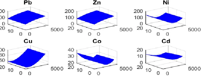
The results of suggested method which illustrate the concentration for each metal given in Figure 1. Also, Figure 2, illustrate the accuracy of suggested method by using a comparison between the results of suggested method, and laboratory dissecting.

The practical results show the following: The average of the concentrations of heavy metals in soil for any time and zones in Alkhuyls city are increase with the time, posing a great risk to the environment contamination.

Table I

Laboratory results where S.M.C. represent of Standard Universal for concentration of heavy metals in soil [22]

measures of heavy metals by

XRF

Fig. 1. concentration of heavy metals by suggested method for Alkhuyls city

1500 day

Fig. 2. Comparing of the concentration calculated by suggested method & XRF

There are different causes for increasing the concentrations of heavy metals in soil such as: the big traffic jams resulting from the great number of cars lately which use gasoline that contains a lot of fourth lead Ethylene which cause big problems to the environment. This creates dangers to human beings. In addition, the increase in the amount of litter and how to get rid of industry waste in sewerage and the decrease in the green region which participate in lessening the damage of heavy metals on the environment. As a result of increase in the population during the late years which results in converting the regions of vegetation to residential regions and the technological development which causes contamination because of the prolife ration of plants and workshops scattered everywhere. Add to all this, wars and their great contamination which are considered the most dangerous contaminates of the soil and environment. All these types of contaminates cause high rate of concentration of heavy metals which exceeds the normal amount in soil, the increase of these

metals has different types of danger on human health. The plants absorb these dangerous materials which in its turn go to human being through food consumption which they acquire because of eating these plants that have the dangerous metals.

7. CONCLUSIONS

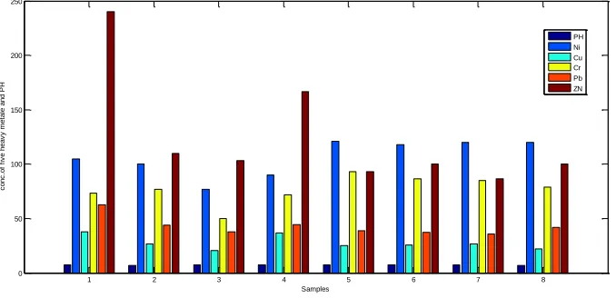
Fig. 3.concentrations of heavy metals in the soils of the different zones in Alkhuyls city

REFERENCES

[1] Burden, L. R., and Faires, J. D., 2001, "Numerical Analysis", Seventh Edition.

[2] Endre Süli and David F. Mayers, 2003, "An Introduction to Numerical Analysis", Cambridge University Press, First published.

[3] Rolf Rannacher, 2007, "Numerische Mathematik 1", Institut für Angewandte Mathematik, Universität Heidelberg Press. [4] Moller, A., Müller, H.W., and Abdullah, A., et al. 2005, "Urban

soil contamination in Damascus, Syria: concentrations and patterns of heavy metals in the soils of the Damascus Ghouta, Geoderma, 124 (1-2), pp:63-71.

[5] Yang, Y.B., and Sun, L.B., 2009, "Status and control countermea sure s of heavy metal pollution in urban soil", Environmental Pprotection Science, Vol.35, No.4, pp: 79-81. [6] Yabe, J., Ishizuka, M., et al., 2010, "Current Levels of Heavy

metal contamination in Africa", Journal of Veterinary Medical Science, Vol.72, No.10, pp: 1257-1263.

[7] Zhang, W.J., Jiang, F.B., and Ou, J.F., 2011, "Global pesticide consumption and pollution: with China as a focus", Proceedings of the International Academy of Ecology and Environmental Sciences, Vol.1, No.2, pp: 125-144.

[8] Sayyed, M.R.G., Sayadi, M.H., 2011, "Variations in the heavy metal accumulations within the surface soils from the Chitgar industrial area of Tehran", Proceedings of the International Academy of Ecology and Environmental Sciences, Vol. 1, No.1, pp: 36-46.

[9] Chen, Y.F., 2011, "Review of the research on heavy metal contamination of China’s city soil and its treatment method", China Population, Resources and Environment, Vol. 21, No. 3, pp: 536-539.

[10] Jean-Philippe, S.R., Labbé, N., Franklin, J.A., et al., 2012, "Detection of mercury and other metals in mercury contaminated soils using mid-infrared spectroscopy", Proceedings of the International Academy of Ecology and Environmental Sciences, Vol. 2, No. 3, pp: 139-149.

[11] Sayadi, M.H., and Rezaei, M.R., 2014, "Impact of land use on the distribution of toxic metals in surface soils in Birjand city, Iran", Proceedings of the International Academy of Ecology and Environmental Sciences, Vol. 4, No. 1, pp: 18-29.

[12] Tawfiq, L. N. M., and Ghazi, F. F., 2015, "Using Artificial Neural Network Technique for the Estimation of Cd Concentration in contaminated Soils", International Journal of Innovations in Scientific Engineering, Vol. 1, No. 1, pp: 1-7.

[13] Tawfiq, L. N. M. and Ghazi, F. F., 2015, "Heavy metals pollution in soil and its influence in Iraq", Merit Research Journal of Agricultural Science and Soil Sciences, Vol. 3, No. 5, pp: 82 - 87.

[14] Tawfiq, L. N. M. and Ghazi, F. F., 2015, "Contaminated Soils by Heavy Metals in South of Iraq", International Journal of Environment and Bioenergy, Vol. 10, No. 3, pp: 41-47. [15] Tawfiq, L. N. M., Kareem A. Jasim and Abdul hmeed, E. O.,

2015, "Pollution of Soils by Heavy Metals in East Baghdad in Iraq", International Journal of Innovative Science, Engineering & Technology, Vol. 2, Issue 6, pp: 181- 187.

[16] Tawfiq, L.N.M., Kareem A. J., and Abdul hmeed, E. O., 2015, "Mathematical Model for Estimation the Concentration of Heavy Metals in Soil for Any Depth and Time and its Application in Iraq", International Journal of Advanced Scientific and Technical Research, Vol. 4, Issue 5, pp:718 – 726.

[17] Tawfiq, L. N. M., and Ghazi, F. F., 2016, "Evaluate the Rate of Contamination Soils by Copper Using Neural Network Technique", Global Journal Of Engineering Science And Researches, Vol. 3, No. 5, pp: 18-22.

[18] Tawfiq, L. N. M., Kareem A. J., and Abdul hmeed, E. O., 2016, "Numerical Model For Estimation The Concentration of Heavy Metals in Soil and Its Application in Iraq", Global Journal of Engineering Science and Researches, Vol. 3, No. 3, PP: 75- 81. [19] Lloyd N. Trefethen, 2006, "Numerical Analysis", Oxford

University Press.

[20] Randall J. LeVeque, 2006, "Finite Difference Methods for Differential Equations", University of Washington Press. [21] Page, A. A., 1986, "Methods Of Soil Analysis, Part 2, Chemical

And Microbiological Properties", 2nd Ed, Madison, Wisconsin, USA: Agronomy, No.9, ASA.

[22] Aziz, F. S., 1989, "Ampient Air Quqlity in Selected Commercial Area in Baghdad City", M.Sc. Thesis, College of Engineering, University of Baghdad.

1 2 3 4 5 6 7 8

0 50 100 150 200 250

Samples

c

o

n

c

.o

f

fi

v

e

h

e

a

v

y

m

e

ta

le

a

n

d

P

H