Theoretical Investigation to Develop a Fit-for-purpose CFD Code to Simulate Transient Incompressible Two-phase Flow

(1)



Abstract — The subject of multiphase flow encompasses a vast field hosting different technological contexts, wide spectrum of different scales and broad range of engineering disciplines along with multitude of different analytical approaches.

A persistent theme throughout the study of multiphase flow is the need to model and predict the detailed behavior of such flow and the phenomenon it manifests. In general, there are three ways to explore the models of multiphase flow:

(1) Develop laboratory-sized models through conducting lab experiments with good data acquisition systems;

(2) Advance theoretical simulations by using mathematical equations and models for the flow; and

(3) Build computer models through utilization of power and size of modern computers to address the complexity of the flow. While full-scale laboratory models are essential to mimic multiphase flow to better understand its boundaries, the predictive capability and physical understanding must depend on theoretical and computational models. Such a combination has always been a major impediment in the industry and academia.

Different numerical methods and models with dissimilar concepts are being conveniently used to simulate multiphase flow systems depending on different concepts. Some of these methods do not respect the balance while others damp down strong gradients. The degree of complexity of these models makes the solution practically not reachable by numerical computations despite the fact that many rigorous and systematic studies have been undertaken so far. The essential difficulty is to describe the turbulent interfacial geometry between the multiple phases and take into account steep gradients of the variables across the interface in order to determine the mass, momentum and energy transfers.

NASA-VOF 3D is a transient free surface fluid dynamics code developed to calculate confined flows in a low gravity environment using the Volume of Fluid (VOF) algorithm. In this study, theoretical investigation has been carried out to better understand the impact of a horizontal bend on incompressible two-phase flow phenomenon. NASA-VOF 3D has been considered as the CFD platform for major modifications carried out to the main two governing equations; namely the Continuity (Mass Conservation) and the Momentum (Navier-Stokes) equations using the Volume of Fluid (VOF) algorithm. The modifications consisted of deriving and developing the governing equations needed to reflect the impact of the bend on the transition. Numerical operators have also been developed to gain better convergence during calculations. This paper presents the details of this theoretical and numerical study and the derivations of the modified governing equations.

Index Terms—CFD, VOF, multiphase flow, horizontal bends, continuity equation, momentum equation.

Manuscript received October 12, 2018; revised December 23, 2018. Amir Alwazzan is with Dragon Oil, Dubai, UAE (e-mail: [email protected]).

I. INTRODUCTION

Hydrocarbons production systems face many challenges from the design to production and decommissioning phases. One of the key challenges is the transport of multiphase streams from the reservoir to the delivery point. Such streams involve phase mixing, rapid changes of flow patterns, mass transfer and phase changes making the systems’ hydrodynamic very complex. Modeling multiphase flow processes is a complex and still developing subject. It is often an iterative process requiring multiple modeling frameworks to understand different aspects of the flow problem. The underlying physics is still inadequately known and a production engineer modeling complex multiphase flow processes often has to complement detailed modeling efforts with validation experiments and field data analysis. It is indeed essential to use a hierarchy of models with an appreciation of “learning” versus “simulation” models to represent multiphase flow processes accurately. An appropriate methodology needs to be developed to systematically interpret the results obtained using different modeling frameworks. Ultimately, there is no substitute for the engineering judgement and creativity of a production engineer to develop a tractable computational model to simulate complex field multiphase flow processes.

All this complexity and chaotic state could lead to operational issues in the production and processing facilities; thus, it is very critical to understand what the expected behavior of the system is and how it would affect the production. From a mathematical point of view, multiphase flow problems are notoriously difficult and much of what we know has been obtained by experimentation and scaling analysis. Not only are the equations, governing the fluid flow in both phases, highly nonlinear, but the position of the phase boundary must generally be found as a part of the solution.

There have been many methods developed in the past few decades to predict multiphase flow behavior in pipes and thousands of papers were published on experiments and modeling of this phenomenon. In most of these cases, models work well for their specific data only.

The key parameters in multiphase flow are flow patterns, pressure gradient, liquid holdup and corrosion related parameters. Due to the dynamic nature of the multiphase flow and the rapid transition among different flow patterns, it is a challenging task to precisely predict these parameters based on extrapolating the base data.

Increasingly sophisticated multiphase flow simulation models have been developed to meet the needs of the

Theoretical Investigation to Develop a Fit-for-purpose

CFD Code to Simulate Transient Incompressible

Two-phase Flow

(2)

operators as they open new frontiers. These models are vital well established tools by which engineers approximate the multiphase flow behavior in wells, piping and flowlines. Using mathematical models built into specialized software programs, flow simulations yield representation of the fluids behavior that might be encountered in a real world of network of wells, flowlines, pipelines and process equipment. The output of these simulations play a prominent role in guiding the operators on the optimum way needed to operate their facilities.

The evolving technique of the CFD (Computational Fluid Dynamics) has gained good advancement as a modelling tool proved to offer good insights on the above issues. CFD is a branch of fluid mechanics that uses numerical analysis and data structures to solve and analyze problems that involve fluid flows. Codes are structured around the numerical algorithms that can tackle fluid flow problems.

They typical procedure to solve a problem using the CFD techniques consists of the following steps:

1. Preparation of the flow data and definition of geometry (Pre-processing);

2. Development of iterative calculation of the flow field by CFD solver;

3. Definition of boundary conditions (definition of property data of fluids and selection of the suitable model);

4. Analysis of calculated results (Post-processing); and 5. Validation of outcomes (compare with experimental data, draw conclusions, re-design and improve process).

CFD solvers are coupled algorithms developed to solve for both continuity and momentum equations at the same time. There are two solution methods for finite volume. These are either with using segregated or coupled solutions. The main difference is that for segregated methods (Lagrangian), one equation for a certain variable is solved for all cells followed by solving the equation for the next variable for all cells and so on. The couple solution methods depends on solving equations for all parameters and variables in a given cell (Eulerian). The segregated solution method is the default method in most commercial finite volume codes. It is best suited for incompressible flows or compressible flows.

There are several numerical techniques in the literature being used to solve the governing equations of simultaneous gas-liquid flow. One of them is the Volume of Fluid (VOF) tracking model. It is a simple, but powerful, free surface modelling numerical technique that is based on the concept of a fractional volume of fluid in a selected cell. The VOF model can model two or more immiscible fluids by solving a single set of momentum equations and tracking the volume fraction of each of the fluids throughout the domain. In other words, VOF is characterized by a mesh that is either stationary or is moving in a certain prescribed manner to accommodate the evolving shape of the interface (Mahady et al. (2015)). This method is proved to be more flexible and efficient than other methods for treating complicated free boundary configurations. The governing equations describing the fluid behaviors, i.e continuity and momentum equations, have to be solved separately and the VOF is not a standalone flow solving algorithm (the same applies for all other advection algorithms). Several recent studies have been carried out by different researchers in the past few years using commercial

packages to deploy the CFD in oil and gas industry (Tocci et al. (2017); Gharaibah et al. (2015) and Khaksarfard et al. (2013)). VOF has been considered in some of these works and the outcomes showed good agreements between measured and calculated values. Lo et al (2010) focused on utilizing two approaches for the turbulence treatment at the gas-liquid interface. Dabirian et al (2015) used the VOF to track the two-phase interface in their work to simulate turbulent flow structure in stratified gas-liquid flow. Yi et al. (2013) used VOF approach to model all the flow regimes, as it allows selective use of surface tension and interface sharpening schemes in an Eulerian framework. Alwazzan (2006 and 2017) presented detailed literature review on the progress of the numerical modeling of the free surfaces and the outcomes of the modified code.

II. GOVERNING EQUATIONS

In solving most of the fluid dynamics problems, two important equations are used; namely the continuity and momentum equations. NASA-VOF 3D program used VOF to solve these two governing equations in one-dimensional linear Cartesian coordinates ((Nichols & Hirt (1980); Hirt & Nichols (1981); Torrey et al. (1985 & 1987) and Mahady et al. (2015)). It is a well-structured code such that individual components can be modified to fit specific problem requirements and/or to accept subsequent code upgrades. Rudman (1997) and Rider & Kothe (1998) presented a comprehensive literature review of the earlier VOF advection methods. This platform has been considered to probe the impact of a horizontal pipe fitting (bend) on the flow pattern transition and pressure variation of incompressible two-phase incompressible flow through major modifications to its governing equations and solving scheme. The conduit description has been considered in the derivation of the governing equations and numerical operators have been developed and introduced to simplify the process.

A. Continuity Equation (Mass Conservation)

The application of conservation of mass to a steady flow in an element results in the equation of continuity, which describes the continuity of the flow from boundary to boundary of the element.

1) Two-dimensional continuity equation – general form

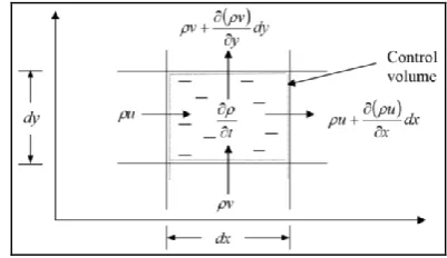
The derivation uses a control volume and the fluid system, which just fills the volume at a particular time t, as shown in Fig. (1) below:

(3)

The control volume is defined as the volume of the full cell. The total mass flow rate stored the fluid element is represented by:

 

0     

 

      

        

dx dy y

v v dy dx x

u u vdx udy dxdy t

  



(1) where u and v are the velocities in the x and y directions, respectively. For incompressible fluid, Equation 1 becomes:

0 











y

x

t



(2)

To convert Equation 2 to cylindrical coordinates, an operator (



) has been developed for simplicity of conversion control as follows:

0 













y

v

x

u

(3)

2) Cylindrical coordinates of a horizontal bend

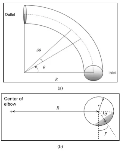
Cylindrical coordinates are combination of polar and Cartesian coordinates. The cross section is polar coordinates, while the axial is Cartesian coordinates, as shown in Fig. 2 below:

(a)

(b)

Fig. 2. (a) Polar coordinate system for a horizontal bend (b)

Cross-section showing tilt of the liquid flowing through a horizontal

bend.

where:

z

,

sin

r

y

,

cos

r

x











(4)

Introducing the functions f and g as:







,



sin

0

0 cos

,













r

y

r

z

y

x

g

r

x

r

z

y

x

f

(5)

Using Jacobian’s matrix and determinant transformation yields:



cos

sin

cos

0 sin

1 













r

g

r

g

f

r

f

g

x

g

f

x

f

x

r

(6)

Similarly;



sin





y

r

(7)

r

x



sin







(8)

r

y



_

cos



(9)

while,

0 ,

1 ,

0 ,

0 



















z

r

z

y

z

x

z



(10)

3) Derivation of the operator of conversion from the cartesian to cylindrical coordinates (



)

In this study, the  operator has been developed and introduced to convert from Cartesian coordinates to cylindrical coordinates. In Cartesian coordinates, vector units are defined as:

z r r

e

k

e

cos

e

sin

j

e

sin

e

cos

i











 



(11)

while in cylindrical coordinates, the vector units are defined

as:-

k

e

j

cos

i

cin

e

j

sin

i

cos

e

r r















 (12)

(4)

chain differentiation:                           _                          _            y z z y y r r e C e S x z z x x r r e S e C z k y j x i r r      





















z

r

e

_z



(13)

Recalling Equations (6) to (10) and using the identity

1

2 sin

2 cos









, Equation (13) could be reduced to:

z

e

r

e

r

e

_r _z

















1

(14)

Using the cylindrical  operator, it gives the gradient of a scalar field

u

:

z r

e

z

u

e

u

r

e

r

u















_



1

(15)

Given the cylindrical vector products:

1 0

0

1          



 r r r z z z z

r e ,e e ,e e ,e e ,e e ,e e

e    

(16)

And the cylindrical vector differentiation identities are:

r r

e

,

e













 (17)

By then, the divergence

 





and Laplacian

 



2 can be worked out for a given field. For a given vector field

z

r

v

e

w

e

u





_



, its divergence becomes:

z z z r r r z r r r r z r z r e e z w e e z v e e z u e e w r e v r e e u r e e e r w e e r v e e r u e w e v e u z e e r e u                                                                   _ _                                1 1 1 (18)

Recalling Equations (16) and (17), we get:

z w e v e v r e e u e u r e r u u r r _                                                

1 1

z

w

v

r

u

r

u



















1

(19) or expressed in more compactly as:

 

z

w

v

r

ru

r

u



















1

(20)

while for Laplacian, (2) operator takes the following form:

z z z r z z r z r r r r z r z r e e z e e z r e e z r e e z r r e r e r e r e e e r z e e r r e e r z e e r e z e e r e                                                                                                         2 2 2 2 2 2 2 2 2 2 1 1 1 1 1 1                 (21) By the same way and from Equations (16) and (17):

2 2 2 2 2 2 2 2

2 1 1

z e e r e e r r e r e r r r                                                   _ _ _ _ _ (22) Thus, 2 2 2 2 2 2 2

2

1

1 z

r





















(23)

For a given scalar field,

u

:

2 2 2 2 2 2 2

2

1

1 z

u

r

u

r

u





















(24)

4) Three-dimensional continuity equation

Following the same approach, Equation (3) could be developed to a three-dimensional one as follows:

0 

















z

w

y

v

x

u

(25)

where u, v and w are the velocities in the x, y and z directions, respectively. For cylindrical coordinates, the following conversion applies:

 

z

w

v

r

ru

r

u



















1

(26)

where u, v and w are the velocities in the radial, azimuthal and axial directions, respectively. The partial cell treatment factor, , could be introduced into Equation (19) resulting:

       



0 





























z

w

y

v

x

u

(27)

 

1  

1    



0 





























z

w

v

r

u

r

u

(5)

5) Introducing the partial cell treatment factor, , into the Continuity and Navier-Stokes equations

The partial cell parameter is treated as one of the properties in the equations. The continuity equation is described as:

0 



















u

(29)

In Cartesian coordinates,

     



0 





















z

w

y

v

x

u

(30)

And for cylindrical  operator,





   

0

1

1 _





























z

w

v

r

u

r

u







(31)

The compact momentum equation for the moving fluid is given by:                                                   

 Ku

P g u u t

u ₍₃₂₎

where  is the volume fraction of the working fluid (that is, the fraction of the volume occupied by the motionless component), K is a coupling constant characterizing the drag between interpenetrating fluid, and



is the viscous stress tensor.

Expanding equation (32) into non-conservative form yields:              _                                  

 Ku

P g u u u u t u t u (33)

The term



















u

in Equation (33) represents the continuity equation. Assuming that the partial cell parameter  is independent of time and incompressible flow; dividing Equation (33) by  gives:

                            u K P g u u t

u ₍₃₄₎

The connection between Equations (29) and (34) and the partial cell treatment is made by specializing  to a situation where  is a step function with values of 0.0 and 1.0 in the obstacle material and moving fluid respectively. First, we note that

u



0 .

0

in the obstacle material and  is constant piecewise. Therefore; the terms in square brackets in Equation (34) can be neglected as the interest is only about the fluid behavior. Hence, the general momentum equation becomes:



























P

g

u

t

u

(35)

Substituting













2

u

and expanding Equation (35), the momentum equations in

x



,

y



and



z

directions become:

                                                                                          2 2 2 2 2 2 2 2 2 2 2 2 2 2 2 2 2 2 1 1 1 z w y w x w z P g z w w y w v x w u t w z v y v x v y P g z v w y v v x v u t v z u y u x u x P g z u w y u v x u u t u z y x       (36) where





 

is the kinematic viscosity,



is the viscosity

and



is the density.

Prior to expressing the momentum equations in cylindrical coordinates, the following transformations are needed:

z r z r r z r z r z r z r z r e z w w e z v w e z u w e w r v e r v e v r v e r uv e u r v e r w u e r v u e r u u e w e v e u z w r v r u e w e v e u z e r e r e e w e v e u u u                                    _ _                      _ _                            _ _                 2 1 z r e z w w w r v r w u e z v w v r v r uv r v u e z u w r v u r v r u u                                                2 (37) z z z z r r r r r r z z z z r r r r z r e z w e w r e r w r e r w e z v e r v e v r e v r e r v r e r v e z u e r u e u r e u r e r u r e r u e z w e w r e r w r e r w e z v e v r e r v r e r v e z u e u r e r u r e r u e w e v e u z r r r r u 2 2 2 2 2 2 2 2 2 2 2 2 2 2 2 2 2 2 2 2 2 2 2 2 2 2 2 2 2 2 2 2 2 2 2 2 2 2 2 2 2 2 2 2 2 2 2 2 2 2 1 1 2 1 1 2 1 1 1 1 1 1 1 1 1 1                                                                                                                   _ _                                          z r e z w w r r w r r w e u r z v v r r v r v r r v e v r z u u r r u r u r r u                                                               2 2 2 2 2 2 2 2 2 2 2 2 2 2 2 2 2 2 2 2 2 2 2 2 2 1 1 2 1 1 2 1 1       (38) From equation (14), the  operator becomes:

(6)

Substituting Equations (37) to (39) into Equation (35) yields the momentum equations in cylindrical coordinates expressed as follows:

                                           v r z u u r r u r u r r u r p g z u w r v u r v r u u t u

r 2 2

2 2 2 2 2 2 2 2 2 1 1 1 (40)                                              u r z v v r r v r v r r v p r g z v w v r v r uv r v u t v 2 2 2 2 2 2 2 2 2 2 1 1 1 (41)                                  2 2 2 2 2 2 2 1 1 1 z w w r r w r r w z p g z w w w r v r w u t w

z _  _



(42)

The derived continuity equations are only applicable to incompressible flow, where the velocity of fluid is less than 30% of the speed of sound.

B. Momentum Equations (Navier-Stokes Equations)

The Equations of Motion (Navier-Stokes equations) can be derived by either applying Newton’s second law to an element of fluid or applying the impulse-momentum principle for control volumes. The derived equations are known to accurately represent the flow physics for Newtonian fluids in very general circumstances, including three-dimensional unsteady flows with variable density. The derived Navier-Stokes equations are applicable to both laminar and turbulent flows and underline much of the practice of modern fluid mechanics. Momentum equations form the basis of the code needed to simulate the system. Their final forms are:

                                                                                                2 2 2 2 2 2 2 2 2 2 2 2 2 2 2 2 2 2 1 1 1 z w y w x w z P g z w w y w v x w u t w z v y v x v y P g z v w y v v x v u t v z u y u x u x P g z u w y u v x u u t u z y x       (43) where ν is the kinematic viscosity, P is the pressure, ρ is the density and gx, gyand gzare the external accelerations in the x,

y and z directions, respectively. The momentum equations in cylindrical coordinates can be written as follows:

                                             v r z u u r r u r u r r u r p g z u w r v u r v r u u t u

r 2 2

2 2 2 2 2 2 2 2 2 1 1 1 (44)                                                u r z v v r r v r v r r v p r g z v w v r v r uv r v u t v 2 2 2 2 2 2 2 2

2 ₁ ₁ ₂

1 (45)                                    2 2 2 2 2 2

2 ₁ ₁

1 z w w r r w r r w z p g z w w w r v r w u t w

z _  _



(46)

where r, θ and z refer to the radial, azimuthal and axial coordinates, respectively. Details of derivations are in Alwazzan (2006).

Equations (44), (45) and (46) are applicable at every point inside the fluid. Once numerically implemented, the arc length azimuthal coordinate y=xIM1θ replaces θ where xIM1 is

the radius of the computational mesh. This emphasizes on the similarity of the derived equations to the Cartesian equations.

C. The Principle of the Fractional Volume-of-fluid (VOF)

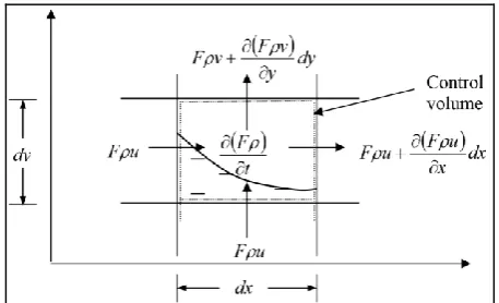
Considering a general free surface cell as indicated in Fig. (3) below:

Fig. 3. Two-dimensional free surface cell that partially filled with fluid

The cell is partially filled with fractional volume-of-fluid (F). The rate of change of mass within the cell is equal to the net flow rate of mass across the element. Hence, the time-dependent of F is governed by the equations:

t

M

st out in







  (47)       dxdy t F dx dy y v F v F dy dx x u F u F vdx F udy F                              (48)

Assuming that the fluid is incompressible and dividing by the area



dxdy



give:

   

t

F

y

Fv

x

Fu













(49)

Expanding Equation (14) yields:

(7)

Note that the square bracket term on the right hand side of Equation (50) is the continuity equation. Hence;

0

~ 

           

F u t F y F v x F u t

F ₍₅₁₎

Using the same procedure, Equation (51) could be developed into three-dimensions as follows:

0 















z

F

w

y

F

v

x

F

u

t

F

(52)

Finally, the transient behavior of gas-liquid flow in a bend can be expressed as follows:

0 













R

H

U

R

U

H

t

H

_L

L L L L

(53)

0 













R

H

U

R

U

H

t

H

_G

G G G G

(54) Using Equation (54) above yields the governing equation for

F in cylindrical coordinates as follows:

0            

z F w F r v r F u t F



(55)

Implementing this approach allows the fluid interfaces to be represented by different equations. However, the flux of F

through each face of the Eulerian grid will be required. Standard finite-difference techniques would lead to a smearing of F values, and the interfaces would lose their definition. Using the step function character of F allows a form of donor-acceptor differencing that preserves the discontinuous nature of F.

III. MODIFIED NASA-VOF3DCODE

NASA-VOF 3D program (Torrey et al., 1987) is a powerful program developed to solve three-dimensional, transient with multiple free boundary two-phase flow. It has a variety of options that provide capabilities for a wide range of applications. It was especially designed to calculate confined flows in a low gas environment, in which surface physics must be accurately treated.

In In this study, NASA-VOF 3D has been considered as the CFD platform to carry out key modifications to the governing equations in order to probe the impact of a horizontal bend on the flow pattern transition during incompressible simultaneous two-phase flow. The modifications consisted of deriving the cylindrical coordinates of the bend and incorporating these changes in the original governing equations. In addition, the volume of fluid algorithm (VOF) has been modified to solve the governing equations for the fluid properties at each cell. The outcomes of the updated

code show good agreement with the experimental data Alwazzan (2017).

REFERENCES

[1] A. Alwazzan, “Developing a 3d CFD code to simulate incompressible simultaneous two-phase flow through a horizontal bend using VOF principle,” International Journal of Engineering and Technology, vol. 9, no. 4, pp. 279-286, August 2017.

[2] A. Alwazzan, “Two-phase flow through horizontal pipe with bend,” PhD Thesis, University of Malaya, KL, Malaysia, 2006.

[3] R. Dabirian, A. Mansouri, R. Mohan, O. Shoham, and G. Kouba, “CFD simulation of turbulent flow structure in stratified gas/liquid flow and validation with experimental data,” SPE-174964-PT, 2015. [4] E. Gharaibah, A. Read, G. and Scheuerer, “Overview of CFD

multiphase flow simulation tools for subsea oil and gas system design, optimization and operation,” OTC Brasil, Rio de Janeiro, Brazil, October 27-29, 2015.

[5] C. W. Hirt and B. D. Nichols, “Volume of fluid (VOF) method for the dynamics of free boundaries,” Journal of Computational Physics,vol. 39, 201-225, 1981.

[6] R. Khaksarfard, M. Paraschivoiu, Z. Zhu, N. Tajallipour, and P. J. Teevens, “CFD based analysis of multiphase flows in bends of large diameter pipelines,” in Proc. CORROSION 2013 NACE International, Orlando, Florida, USA, March 17-21, 2013.

[7] H. S. Kwak and K. Kuwahara, “A VOF-FCT method for simulating two-phase flows on immiscible fluids,” The Institute of Space and Astronautical Science, 1996.

[8] S. Lo and A. Tomasello, “Recent progress in CFD modelling of multiphase flow in horizontal and near-horizontal pipes,” in Proc. 7th N. American Conference on Multiphase Technology, Banff, Canada, June 2-4, 2010.

[9] K. Mahady, S. Afkhami, and L. Kondic, “A volume fluid method for simulating fluid/fluid interfaces in contact with solid boundaries,” Journal of Computational Physics, vol. 294, pp. 243–257, 2015. [10] B. D. Nichols, C. W. Hirt, and R. S. Hotchkiss, “SOLA-VOF: A

solution logarithm for transient fluid flow with multiple free boundaries,” Technical Report LA-8355, Los Alamos National Laboratory, 1980.

[11] W. J. Rider and D. B. Kothe, “Reconstructing volume tracking,” Journal of Computational Physics, vol. 141, pp. 112-152, 1998. [12] M. Rudman, “Volume-tracking methods for interfacial flow

calculations,” International Journal for Numerical Methods in Fluids, vol. 24, pp. 671-691, 1997.

[13] F.T occi, F. Bos, and R. Henkes, “CFD for multiphase flow in vertical risers,” in Proc. 18th_{International Conference on Multiphase}

Production Technology, France, June 7-9, 2017.

[14] M. D. Torrey, L. D. Cloutman R. C. Mjolsness, and C. W. Hewit, “NASA-VOF2D: A computer program for incompressible flows with free surfaces,” Technical Report LA-10612-MS, Los Alamos National Laboratory, 1985.

[15] M. D. Torrey, R. C. Mjolsness, and L. R. Stein, “NASA-VOF3D: A three dimensional computer program for incompressible flows with free surfaces,” Technical Report LA-11009-MS, Los Alamos National Laboratory, 1987.

[16] D. Yi, D. Duraivelan, and A. Madhusuden, “CFD modeling of bubbly, slug and annular flow regimes in vertical pipelines,” OTC, Houston, Texas.