Manuscript Title & Authors

e-ISSN: 2278-7461, p-ISSN: 2319-6491

Volume 6, Issue 2 (Feb 2017) PP: 37-53

Effect of joule heating on mixed convection flow of Casson

nanofluid over a non-linear permeable stretching sheet with heat

generation or absorption

Dasaradha Ramaiah K.

Ranga Rao T.

and K. Gangadhar

1_{Department of Mathematics, Dhanekula Institute of Engineering and Technology, Ganguru-521139, Andhra}

Pradesh, India

2

Department of Mathematics, SVKP College, Markapur, Prakasam, India

3_{Department of Mathematics, Acharya Nagarjuna University, Ongole, Andhra Pradesh -523001, India}

ABSTRACT:- In this paper, numerical analysis has been carried out on the problem of magnetohydrodynamic (MHD) mixed convection flow of a Casson nanofluid past a nonlinear permeable stretching sheet with viscous dissipation in the presence of double stratification, joule heating. The governing partial differential equations are transformed into a system of ordinary differential equations using suitable similarity transformations. The resultant ordinary differential equations are then solved numerically by bvp 4c Matlab software. Effects of the physical parameters on the velocity, temperature and concentration profiles as well as the local skin friction coefficient, the heat and mass transfer rates are depicted in tabular form and discussed. The results indicate that the local Nusselt number decreases with an increase in both Brownian motion parameter Nb and the thermophoresisparameter Nt. However, the local Sherwood number increases with an increase in Brownian motion parameter Nb. But it decreases as the values of Nt increases. Besides it is found that the surface temperature of sheet increases with an increase in the heat generation (Q>0) or absorption parameter (Q<0). Comparison of present results with previously reported results has been found in excellent agreement.

Keywords: Nonlinear permeable stretching sheet, MHD, Joule heating, Casson nanofluid , double stratification.

I.

INTRODUCTION

rejection into the environment such as lakes, rivers, and seas; thermal energy storage systems such as solar ponds; and heat transfer from thermal sources such as the condensers of power plants. Although the effect of stratification of the medium on the heat removal process in a fluid is important, very little work has been reported in literature [39-42]. Srinivasacharya and Upendar [43] considered the flow and heat and mass transfer characteristics of the free convection on a vertical plate with variable wall temperature and concentration in a doubly stratified micropolar fluid where they concluded that an increase in thermal (solutal) stratification parameter reduces the velocity, temperature (concentration), skin friction, heat and mass transfer rates but enhance the concentration (temperature) and wall couple stress. Motivated by the above investigations the present paper, numerical analysis has been carried out on the problem of magnetohydrodynamic (MHD) mixed convection flow of a Casson nanofluid past a nonlinear permeable stretching sheet with viscous dissipation in the presence of double stratification and heat generation or absorption. The governing partial differential equations are transformed into a system of ordinary differential equations using suitable similarity transformations. The resultant ordinary differential equations are then solved numerically through computer software. Effects of the physical parameters on the velocity, temperature and concentration profiles as well as the local skin friction coefficient, the heat and mass transfer rates are depicted in tabular form and discussed.

II.

MATHEMATICAL FORMULATION

Let us consider the two dimensional steady incompressible flow of a Casson nanofluid induced by a nonlinearly stretching sheet which is placed at y=0. The flow is confined to y >0. By keeping the origin is fixed

and sheet is stretched with nonlinear velocityu_w  a xn , where a is positive constant, n>0 for an accelerated sheet and n<0 for a decelerated sheet. The stretching sheet is assumed to be coinciding with the x − axes while the y − axis is perpendicular to the plane of the sheet. The surface is maintained at temperature T_w

 

 

 

 

1

B are constants and varied to alter the intensity of stratification in the medium and T_{, 0} and C_{, 0} are the beginning ambient temperature and nanoparticle volume fraction at x  0 respectively.

The rheological equation of state for an isotropic flow of a Casson fluid (Eldabe and Salwa [14] can be expressed as

2 ,

2

2 ,

2

y

B i j c

y

B i j c

c

p

e

i j _p

e

  



  





 

 

 

 

 

   

 

 











(2.1)

where 𝜇𝐵 is plastic dynamic viscosity of the non-Newtonian fluid, 𝑝𝑦 is the yield stress of fluid, 𝜋 is the product

of the component of deformation rate with itself, namely, 𝜋 = 𝑒𝑖𝑗𝑒𝑖𝑗, 𝑒𝑖𝑗 is the (𝑖, 𝑗)th component of the

deformation rate, and 𝜋𝑐 is critical value of 𝜋 based on non-Newtonian model. A magnetic field is applied in

the direction perpendicular to the sheet with varying strength as a function of x. The flow region is exposed under uniform transverse magnetics fields 𝐵 = (0, B(x), 0) and uniform electric field 𝐸 = (0, 0, −𝐸0). Since

such imposition of electric and magnetic fields stabilizes the boundary layer flow. It is assumed that the flow is generated by stretching of an elastic boundary sheet from a slit by imposing two equal and opposite forces in such a way that velocity of the boundary sheet is of linear order of the flow direction. We know from Maxwell‟s equation that ∇. 𝐵 =0 and ∇. 𝐸 = 0 . When magnetic field is not so strong then electric field and magnetic field obey Ohm‟s Law 𝐽 = 𝜎(𝐸 + 𝑞 × 𝐵 ) , where is the Joule current, 𝜎is the magnetic permeability and 𝑞 is the fluid velocity. We assume that magnetic Reynolds number of the fluid is small so that induced magnetic field and Hall effect may be neglected. We take into account of magnetic field effect as well as electric field in momentum and thermal boundary layer equations. By implementing the boundary layer approximations and applying the order of magnitude analysis, the governing equations (2.2) to (2.5) are transformed into the following equations:

0

u v

x y

 

 









2

2 0

2

1

1 ( ) ( ) _T( ) _C( )

u u u

u v E B x B x u g T T C C

x y y



  

   

 

  

  _  _      

  _{ }  (2.3)









2 2

2

2

2 0 0

1

1 ( )

T B

P p p

T T T C T D T

u v D

x y y y y T y

Q u

u B x E T T

C y C C

 

 

   





 _{ } 

     

     _{ } 

   _   _  _{ }

 

  

 _  _{ }    



   

(2.4)

2 2

2 2

T B

C C C D T

u v D

x y y T_ y

 

   

  _{  }

   _{ }  (2.5)

The boundary conditions for velocity, temperature and concentration fields are

, ,

0 : _w n, _{w w w}

y  u  a x v  v T  T C  C

0 : 0 , 0 , , ,

y  u  v  T  T_ C  C_ (2.6)

Where u and v are the velocity component along the x and y axes respectively,





k C 



 is the

thermal diffusivity, is the kinematic viscosity,  is dynamic viscosity of the fluid, , is vortex viscosity, 

is fluid density, is the Casson fluid parameter,_f is the density of base fluid, g is the acceleration due to

gravity,_T is coefficient of thermal expansion,_C is the coefficient of expansion with concentration, D_B is the Brownian diffusion coefficient, D_T is the thermophoresis diffusion coefficient,Q₀ is the heat generation or

absorption coefficient ,









p

f C C  



 is the ratio of nanoparticle heat capacity and base fluid heat capacity

,C is the volumetric volume coefficient,_p is the density of the particles and c is the rescaled nanoparticl, k p is

the permeability of the porous medium, σ is the electrical conductivity, B0 is the magnetic field strength, cp is

the specific heat at constant pressure and m is the heat flux exponent. We assume that It is noted here that the case of uniform surface heat flux corresponds to m = 0.

Following [15, 16, 17], the strength of the spatially varying magnetic field B(x) is taken as

B(x)=B0x(n−1)/2 (2.7)

where B0 is the strength of the magnetic field.

𝜓(𝑥, 𝑦) is the stream function defined in the usual way as

u y 

 

 and v x



  

 (2.8)

So that the conservation of mass equation (2.2) is automatically satisfied. Now, we introduce the following similarity transformations





 





 

 

 

1 1

2 2

1 1 1

, ' ,

2 2 1

n n

n

a n a n n

y x u a x f x f f

n 

     



 

    

    _  _



  (2.9)

The dimensionless temperature and concentration are

 

2 , 0 1

T T A x

T T

     

  ,

 

2 , 0 1 w

T T x T_ M x

   

. (2.10)

 

2 , 0 1

C C B x

C C

   

 

  ,

 

2 , 0 1 w

C C x C_ N x

and assume





2 1 2 n w w a n x f    

  ,where fw is the suction or injection parameter.

After the substitution of these transformations (2.7) - (2.11) along with the equations (2.2) – (2.6) the resulting non-linear ordinary differential equations are written as follows:





1

1 2

(1 ) ' ( ') 0

1

f ff n f G r G c M E f

n

 

  

       

 (2.12)





2 2 2

1 1

1 1

" ' ' ' ' 1 '' ( ' ) ' 0

P r t

f N b N E c f E c M f E Q f

              _  _        (2.13) 2

'' P r ' t '' ' 0 .

b N

L e f f

N

      

(2.14) The corresponding boundary conditions are

1 2

( 0 ) _w, '( 0 ) 1, ( 0 ) 1 , ( 0 ) 1

f  f f       

 

 

 

' 0 , 0 , 0

f         (2.15)

Where prime denotes differentiation with respect to . The Physical parameters involved in the above equations

are defined as P r  

 is Pradantl number,

B L e

D 

 is Lewis number,



 







B w p

b

f

D C C C

N C     

 is the

Brownian motion parameter, ,



 







T w p

t

f

D T T C

N T C      

 is the thermophoresis parameter,

0 /

M  B  a is magnetic parameter, E₁  E₀ /B a x₀ ( 3n1 ) / 2 is the local electric parameter,





C T T_ 

 is Eckert number,





2 2 1 T w

n

g T T

G r

a x

 _





 is called local Grashof number ,





2 2 1 C w

n

g C C

G c

a x

 _





 is the local modified Grashof number, 0 p Q Q

C a 

 is the heat generation (Q>0) or

absorption (Q<0) parameter,

 

2

1

x d

T x T d x

  _{ } _

 is the thermal stratification parameter and

 

2

2

x d

C x C d x

  _{ } _

 is the solutal stratification parameter.

The quantities of the skin friction coefficient 𝐶𝑓 , the local Nusselt number 𝑁𝑢𝑥 and the local Sherwood number 𝑆ℎ𝑥 given as follows

2 w f w C u    where 0 1 1 w B y u y    _       _  _{ }      ,





k T T

  ,





D C C





(2.16)

where k is the thermal conductivity of the nano fluid and qw,qm _{are the heat and mass fluxes at the} surface respectively given by

0

,

w m B

y o y

T C

q k q D

y _ y _

    

  _{ }   _{ }

 

    (2.17)

 

 

 

1 / 2 1 1 / 2 1 1 / 2 1

R e 1 '' 0 , R e ' 0 , R e ' 0

2 2

x f x x x x

n n

C f N u  S h 



 

   

_  _    

 

Where R e w x

u x 



which is called local Reynolds number.

III.

SOLUTION OF THE PROBLEM

The system of ordinary differential equations (2.12)-(2.14) along with the boundary condition

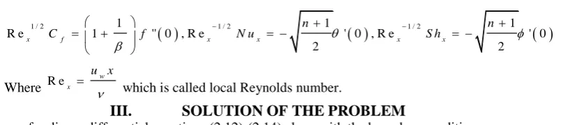
(2.15) are integrated numerically by first choosing initial guess values for f( 0 ) , f ''( 0 ) , '( 0 ) and  '( 0 ) to match the boundary conditions at . Matlab bvp4c solver (ref. Shampine and Kierzenka [18]) was used to integrate the system of equations. To verify the accuracy of the numerical results, we compared our results with those reported by Besthapu and Bandari [19], Mabood et al. [5], Rana and Bhargava [20] as shown in table 1. The results are in very good agreement, thus lending confidence to the accuracy of the present results.

IV.

RESULTS AND DISCUSSION

In order to get physical understanding, the numerical values of the parameters encountered in the problem are valid and there by the velocity, temperature and nanoparticle volume fraction (nanoparticle concentration) profiles have been discussed. Graphical illustrations are given to the tabulated numerical results.

The controlling parameters are taken as β = 0.5, n=2, Gr = 0.2, Gc = 0.2, Pr = 0.71, Nt = 0.2, Nb = 0.2, Ec = 0.5, Le = 2, fw = 1.5, Q = 0.2, 𝜀1= 0.1 & 𝜀2 = 0.2, discussed the effect of magnetic parameter, the effect of

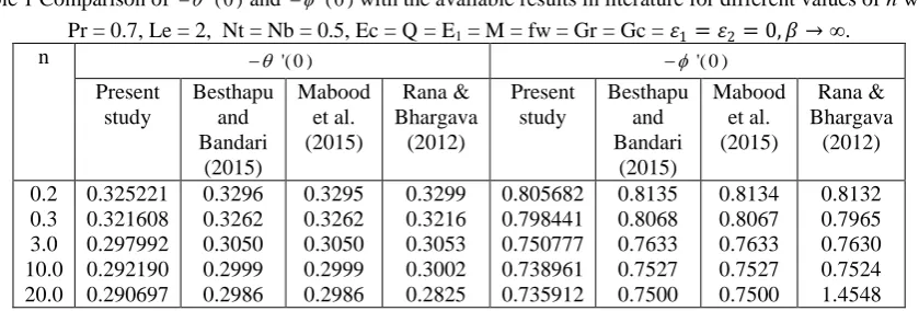
magnetic parameter (M) on dimensionless velocity, temperature and nanoparticle volume fraction profiles are showed in figures 1(a) and 2(b) respectively. As the increase in magnetic parameter, the non-dimensional velocity profile is decreased. This is due to the in introduction of a transverse magnetic field which is normalto the flow direction and has a tendency to create the drag known as Lorentz force, tends to resist the flow. Hence, as the magnetic parameter increases, there is a decrease in the horizontal velocity profiles (see in fig.1(a)). From figure 1(b), we define the thermal energy as the additional force which drags the nanofluid from the influence of magnetic field. This additional force increases the thickness of the thermal boundary layer, so that the temperature profiles enhances with the rise of magnetic parameter values. From this figure, we have observed that as the values of M increases, the volume fraction of nanoparticle distributions is also enriched in the flow region. Figures 2(a) and 2(b) illustrate the effect of thermal Grashof number (Gr) on dimensionless velocity, temperature and nanoparticle volume fraction profiles. The other parameters are fixed as M=0.5, β = 0.5, n=2, Gc = 0.2, Pr = 0.71, Nt = 0.2, Nb = 0.2, Ec = 0.5, Le = 2, fw = 1.5, Q = 0.2, 𝜀1= 0.1 & 𝜀2 = 0.2. Thermal

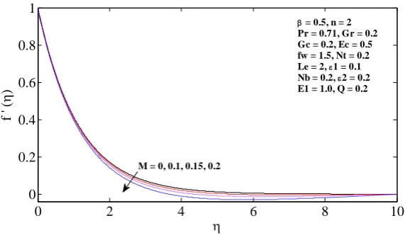
Grashof number represents the ratio of the buoyancy force to the viscous force acting on the fluid. It is observed that on increasing the thermal Grashof number, the dimensionless velocity significantly increased. Evidently, thickness of thermal and nanoparticle volume fraction boundary layers significantly decrease larger distance from the surface as the thermal Grashof number is increased. The effect of solutal Grashof number (Gc) on the dimensionless velocity, temperature and concentration fields are depicted in figures 3(a) and 3(b) respectively. The other controlling parameters are set to be constant at M=0.5, β = 0.5, n=2, Gr = 0.2, Pr = 0.71, Nt = 0.2, Nb = 0.2, Ec = 0.5, Le = 2, fw = 1.5, Q = 0.2, 𝜀1= 0.1 & 𝜀2 = 0.2. It is observed that as the solutal Grashof number

increases, the velocity remarkably increases; while the solutal Grashof number increases, the temperature and nanoparticle volume fraction distributions are decreased. The other controlling parameters are set to be constant at M=0.5, β = 0.5, n=2, Gr = 0.2, Gc = 0.2, Pr = 0.71, Nt = 0.2, Nb = 0.2, Ec = 0.5, Le = 2, Q = 0.2, 𝜀1=

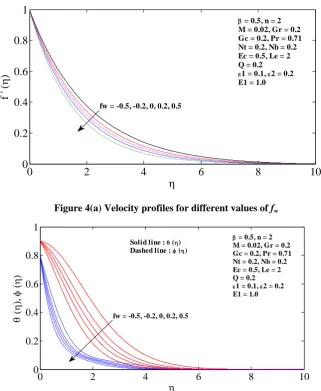
0.1 & 𝜀2 = 0.2. Figures 4(a) & 4(b) exemplifies the effect of suction or injection parameter (fw) on the

dimensionless velocity, temperature and concentration distributions respectively. As depicted in figure 4(a), the velocity distribution is decreased by suction parameter (f w >0) where as it is increased by injection parameter (f

w < 0). It is obvious that imposed suction decreases the boundary layer thickness. In other words, imposed injection increases the velocity distribution in the boundary layer region. Thus it signifies that injection parameter helps the flow to penetrate more into the fluid. Figure 4(b) demonstrate the suction (f w>0) decrease the temperature and injection (f w <0) increase the temperature throughout the boundary layer. It can be viewed that suction will lead to fast cooling of the surface. This is remarkably important in numerous industrial applications. Further, it is noted that the surface receives heat due to injection parameter and from the surface for suction. Moreover, it is observed that the temperature increase near the surface due to injection and decreases until its value become zero at the outside of the boundary layer. Figure 4(b) demonstrates that suction parameter (f w>0) decreases the nanoparticle volume fraction distribution where as injection parameter increases it. Figures 5(a) and 5(b) describe the effect of Casson parameter (β) on the dimensionless velocity, temperature and concentration profiles. The other controlling parameters are set to be constant at M=0.5, n=2, Gr = 0.2, Gc = 0.2, Pr = 0.71, Nt = 0.2, Nb = 0.2, Ec = 0.5, Le = 2, fw = 1.5, Q = 0.2, 𝜀1= 0.1 & 𝜀2 = 0.2. It is

𝛽 →∞,1

𝛽→ 0, the fluid becomes Newtonian. It is noticed that the rise in the values of Casson parameter is used

to dilute the strength of yield stress Py of the Casson fluid which enhances the value of plastic dynamic viscosity 𝜇𝐵 and causing the resistance in fluid flow. On increasing the Casson parameter is to increase the fluid

non-dimensional temperature and nanoparticle volume fraction profiles is observed. The phenomenon in which the particles can diffuse under the effect of a temperature gradient is called thermophoresis. The influence of thermophoresis parameter (Nt) on dimensionless temperature and nanoparcle volume fraction profiles can be viewed in figure 6 respectively. The other controlling parameters are set to be constant at M=0.5, β = 0.5, n=2, Gr = 0.2, Gc = 0.2, Pr = 0.71, Nb = 0.2, Ec = 0.5, Le = 2, fw = 1.5, Q = 0.2, 𝜀1= 0.1 & 𝜀2 = 0.2. It is observed

that temperature and nanoparticle volume fraction profiles elevate in the boundary layer region with the higher values of thermophoresis parameter (Nt). This is from the reality that particles near the hot surface create thermophoretic force; this force enhances the temperature and volume fraction of nanoparticles of the fluid in the boundary layer region. The random motion of nanoparticles within the base fluid is called Brownian motion which occurs due to the continuous collisions between the nanoparticles and molecules of the base fluid. Figures 7(a) and 7(b) shows the effects on velocity, temperature and nanoparticle volume fraction profiles for various values of Brownian motion parameter (Nb). The effect of Brownian motion parameter Nb are explicated by setting the values of other parameters to be constant at M=0.5, β = 0.5, n=2, Gr = 0.2, Gc = 0.2, Pr = 0.71, Nt = 0.2, Ec = 0.5, Le = 2, fw = 1.5, Q = 0.2, 𝜀1= 0.1 & 𝜀2 = 0.2. It is noticed that temperature profiles are increased

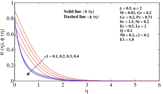
when Brownian motion parameter Nb increases. The physics behind the rise in temperature is that the increased Brownian motion parameter increases of the thickness of the thermal boundary layer. However, in the case of nanoparticle volume fraction, it results in a decrease while Brownian motion parameter is increased away from the surface.In order to discuss the influence of thermal stratification parameter(𝜀1), the other parameters are set

constantly at M=0.5, β = 0.5, n=2, Gr = 0.2, Gc = 0.2, Pr = 0.71, Nt = 0.2, Nb = 0.2, Ec = 0.5, Le = 2, fw = 1.5, Q = 0.2 & 𝜀2 = 0.2. From figures 8, it is noted that on increasing thermal stratification parameter, the thermal and

volume fraction of nanoparticles boundary layers decreases. From this, it is evidently seen that the thermal stratification tends to delay the thermal boundary layer flow process. Moreover, it will have some practical implications on the heat transfer amplification process.The other parameters are set as M=0.5, β = 0.5, n=2, Gr = 0.2, Gc = 0.2, Pr = 0.71, Nt = 0.2, Nb = 0.2, Le = 2, fw = 1.5, 𝜀1= 0.1 & 𝜀2 = 0.2.The influence of Eckert

number (Ec) and heat generation (Q>0) or absorption (Q<0) parameter on the temperature profiles within the boundary layer region is shown in the figure 9. As compared to the case of absence of viscous dissipation, it is understood that the temperature profile is increased on increasing the Eckert number. Due to viscous heating, the increase in the fluid temperature is enhanced and appreciable for higher values of Eckert number. In other words, increasing the Eckert number leads to a coolness of the wall. Consequently, a heat transfer of heat to the fluid occurs, which causes a rise in the temperature of a fluid. From figure 9, we can be observed that the effect of heat absorption results in a fall of temperature since heat resulting from the wall is observed. Obviously, the heat generation leads to an increase in temperature throughout the entire boundary layer. Furthermore, it should be noted that for the case of heat generation, the fluid temperature becomes maximum in the fluid layer adjacent to the wall rather at the wall. In fact, the heat generation effect not only has the tendency to increase the fluid temperature but also increases the thermal boundary layer thickness. Due to heat absorption, it is observed that the fluid temperature as well as the thermal boundary layer thickness is decreased. No significance in heat distribution is observed among the fluids in the presence of heat absorption. The other parameters are set as M=0.5, β = 0.5, n=2, Gr = 0.2, Gc = 0.2, Nt = 0.2, Nb = 0.2, Ec = 0.5, Le = 2, fw = 1.5, Q = 0.2, 𝜀1= 0.1 & 𝜀2 =

0.2. The effect of Prandtl number (Pr) on temperature profiles is illustrated in figure 10. It can be observed that the temperature profile is decreased on increasing Prandtl number. The ratio between momentum diffusivity and thermal diffusivity of the fluid is known as Prandtl number. Physically, Pr = 0.68 refers to Helium, Pr = 0.71 corresponds to air, Pr = 5.1 refers to water and Pr = 12.3 corresponds to Ethylene Glycol 30%. Increasing Prandtl number becomes a key factor to reduce the thickness of the thermal boundary layer. Setting the other parameters to be constant as M=0.5, β = 0.5, n=2, Gr = 0.2, Gc = 0.2, Pr = 0.71, Nt = 0.2, Nb = 0.2, Ec = 0.5, fw = 1.5, Q = 0.2, 𝜀1= 0.1. The discussion is now made only by varying the solutal stratification parameter (ε2) and Lewis number (Le).The effect for the variation of solutal stratification parameter on the concentration profile is exemplified in figure 11. It is confirmed that the concentration distribution is significantly decreased while the values of solutal stratification parameter and Lewis number is increased.

Table 2 shows that the Skin friction coefficient, Local Nusselt number and Local Sherwood number

(which are respectively proportional to 1 1 ''( 0 ) , 1 '( 0 ) & 1 '( 0 )

2 2

n n

f  



     

   

   

 _{ } 

 

for different

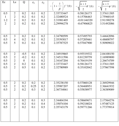
solutal Grashof number strictly decreases the value of both skin friction coefficient and local Sherwood number while local Nusselt number increases. The skin friction coefficient, local Nusselt number and local Sherwood numbers are significantly decreased by increasing the non linear stretching parameter and suction or injection parameter. On increasing the Brownian motion parameter or magnetic parameter strictly increases the values of both skin friction coefficient and local Sherwood number where as local Nusselt number decreased. Moreover, the local Nusselt number and local skin friction coefficient are increased on increasing the Prandtl number while the local Sherwood number decreases. This signifies that a fluid with larger Pr possess larger heat capacity and hence improves the heat transfer. On the other hand, the skin friction coefficient, local Nusselt number and local Sherwood number are decreased by increasing the thermophoresis parameter. Table 3 illustrates that the effect of viscous dissipation, Lewis number, heat generation or absorption parameter, thermal stratification parameter and solutal stratification parameter on the local skin friction coefficient, local Nusselt number and local Sherwood number. It is observed that increasing Eckert number or heat generation or absorption parameter significantly decreases the skin friction coefficient and rate of heat transfer whereas rate of mass transfer is increased. On increasing the Lewis number, slight decrease in the rate of heat transfer and slight increase in skin friction coefficient and mass transfer rate are observed. When thermal stratification number is increased, skin friction coefficient is significantly increased and a decrease in the rate of heat and mass transfer can be noticed. The skin friction coefficient heat transfer rate is increased but mass transfer rate decreased on increasing the solutal stratification parameter.

V.

CONCLUSION

In this paper, a numerical investigation has been carried out to discuss the double stratification and heat generation or absorption effects on magneto hydrodynamic mixed convection flow of a Casson nanofluid over a nonlinear permeable stretching sheet under the influence of viscous dissipation. The concluding facts for the present work after a thorough observation are briefed as follows

1.On increasing magnetic parameter or Casson fluid parameter and simultaneously decreasing buoyancy parameters (Gr, Gc) in a significant decrease of the momentum boundary layer thickness whereas the thermal and concentration boundary layer thickness increases of the fluid.

2.Thickness of the thermal and concentration boundary layers significantly increases away from the surface where the thermophoresis parameter increases.

3.When the Brownian motion parameter increases, the thermal boundary layer thickness increases where as concentration boundary layer thickness decreases.

4.On increasing thermal stratification parameter results in significant decrease of the thermal and concentration boundary layer thickness.

5.From low thermal stratification to high thermal stratification, Skin friction coefficient increases whereas local Nusselt and Sherwood number increased.

6.From low solutal stratification parameter to high solutal stratification parameter, the skin coefficient and local Nusselt number are increased whereas mass transfer rate decreased.

Table 1 Comparison of  '( 0 )and  '( 0 )with the available results in literature for different values of n when Pr = 0.7, Le = 2, Nt = Nb = 0.5, Ec = Q = E1 = M = fw = Gr = Gc = 𝜀1= 𝜀2= 0, 𝛽 →∞.

n _{ '( 0 ) '( 0 )}

Present study

Besthapu and Bandari

(2015)

Mabood et al. (2015)

Rana & Bhargava

(2012)

Present study

Besthapu and Bandari

(2015)

Mabood et al. (2015)

Rana & Bhargava

(2012)

0.2 0.3 3.0 10.0 20.0

0.325221 0.321608 0.297992 0.292190 0.290697

0.3296 0.3262 0.3050 0.2999 0.2986

0.3295 0.3262 0.3050 0.2999 0.2986

0.3299 0.3216 0.3053 0.3002 0.2825

0.805682 0.798441 0.750777 0.738961 0.735912

0.8135 0.8068 0.7633 0.7527 0.7500

0.8134 0.8067 0.7633 0.7527 0.7500

Figure 1(a) Velocity profiles for different values of M

Figure 1(b) Temperature profiles (Solid line) and Concentration profiles (Dashed line) for different values of M

Figure 2(a) Velocity profiles for different values of Gr

0 2 4 6 8 10

0 0.2 0.4 0.6 0.8 1



f '

(



)

 = 0.5, n = 2 Pr = 0.71, Gr = 0.2 Gc = 0.2, Ec = 0.5 fw = 1.5, Nt = 0.2 Le = 2, 1 = 0.1 Nb = 0.2, 2 = 0.2 E1 = 1.0, Q = 0.2

M = 0, 0.1, 0.15, 0.2

0 2 4 6 8 10

0 0.2 0.4 0.6 0.8 1





(



),



(



)

 = 0.5, n = 2

Pr = 0.71, Gr = 0.2 Gc = 0.2, Ec = 0.5 fw = 1.5, Nt = 0.2

Le = 2, 1 = 0.1

Nb = 0.2, 2 = 0.2

E1 = 1.0, Q = 0.2

M = 0, 0.1, 0.15, 0.2

Solid lie :  () Dashed line :  ()

0

2

4

6

8

10

0

0.2

0.4

0.6

0.8

1



f '

(



)

Gr = 0, 2, 4, 6

Figure 2(b) Temperature profiles (Solid line) and Concentration profiles (Dashed line) for different values of Gr

Figure 3(a) Velocity profiles for different values of Gc

Figure 3(b) Temperature profiles (Solid line) and Concentration profiles (Dashed line) for different values of Gc

0

1

2

3

4

5

6

0

0.2

0.4

0.6

0.8

1





(



),



(



)

Gr = 0, 2, 4, 6

Solid line :  () Dashed line :  ()

 = 0.5, n = 2 M = 0.02

Gc = 0.2, Pr = 0.71 Nt = 0.2, Nb = 0.2 Ec = 0.5, Le = 2 fw = 1.5, Q = 0.2 1 = 0.1, 2 = 0.2 E1 = 1.0

0 2 4 6 8 10

0 0.2 0.4 0.6 0.8 1



f '

(



)

Gc = 0, 2, 4, 6

 = 0.5, n = 2

M = 0.02 Gr = 0.2, Pr = 0.71 Nt = 0.2, Nb = 0.2 Ec = 0.5, Le = 2 fw = 1.5, Q = 0.2

1 = 0.1, 2 = 0.2

E1 = 1.0

0

1

2

3

4

5

6

0

0.2

0.4

0.6

0.8

1





(



),



(



)

Solid line :  () Dashed line :  ()

 = 0.5, n = 2 M = 0.02

Gr = 0.2, Pr = 0.71 Nt = 0.2, Nb = 0.2 Ec = 0.5, Le = 2 fw = 1.5, Q = 0.2 1 = 0.1, 2 = 0.2 E1 = 1.0

Figure 4(a) Velocity profiles for different values of fw

Figure 4(b) Temperature profiles (Solid line) and Concentration profiles (Dashed line) for different values of fw

Figure 5(a) Velocity profiles for different values of β

0

2

4

6

8

10

0

0.2

0.4

0.6

0.8

1



f '

(



)

 = 0.5, n = 2

M = 0.02, Gr = 0.2 Gc = 0.2, Pr = 0.71 Nt = 0.2, Nb = 0.2 Ec = 0.5, Le = 2 Q = 0.2

1 = 0.1, 2 = 0.2

E1 = 1.0

fw = -0.5, -0.2, 0, 0.2, 0.5

0 2 4 6 8 10

0 0.2 0.4 0.6 0.8 1





(



),



(



)

Solid line :  () Dashed line :  ()

fw = -0.5, -0.2, 0, 0.2, 0.5

 = 0.5, n = 2 M = 0.02, Gr = 0.2 Gc = 0.2, Pr = 0.71 Nt = 0.2, Nb = 0.2 Ec = 0.5, Le = 2 Q = 0.2

1 = 0.1, 2 = 0.2 E1 = 1.0

0 2 4 6 8 10

0 0.2 0.4 0.6 0.8 1



f '

(



)

fw = 1.5, n = 2 M = 0.02, Gr = 0.2 Gc = 0.2, Pr = 0.71 Nt = 0.2, Nb = 0.2 Ec = 0.5, Le = 2 Q = 0.2

1 = 0.1, 2 = 0.2 E1 = 1.0

Figure 5(b) Temperature profiles (Solid line) and Concentration profiles (Dashed line) for different values of β

Figure 6 Temperature profiles (Solid line) and Concentration profiles (Dashed line) for different values of

Nt

Figure 7 Temperature profiles (Solid line) and Concentration profiles (Dashed line) for different values of

Nb

0

1

2

3

4

5

6

0

0.2

0.4

0.6

0.8

1





(



),



(



)

Solid line :  ()

Dashed line :  ()

Nt = 0.2, n = 2 M = 0.02, Gr = 0.2 Gc = 0.2, Pr = 0.71 fw = 1.5, Nt = 0.2 Ec = 0.5, Le = 2 Q = 0.2

1 = 0.1, 2 = 0.2

E1 = 1.0

 = 0.5, 1, 2, 

0

1

2

3

4

5

6

0

0.2

0.4

0.6

0.8

1





(



),



(



)

Solid line :  ()

Dashed line :  ()

 = 0.5, n = 2

M = 0.02, Gr = 0.2 Gc = 0.2, Pr = 0.71 fw = 1.5, Nb = 0.2 Ec = 0.5, Le = 2 Q = 0.2

1 = 0.1, 2 = 0.2

E1 = 1.0

Nt = 0.1, 0.3, 0.5, 0.7

0

1

2

3

4

5

0

0.2

0.4

0.6

0.8

1





(



),



(



)

Solid line :  ()

Dashed line :  ()

 = 0.5, n = 2

M = 0.02, Gr = 0.2 Gc = 0.2, Pr = 0.71 fw = 1.5, Nt = 0.2 Ec = 0.5, Le = 2 Q = 0.2

1 = 0.1, 2 = 0.2

Figure 8 Temperature profiles (Solid line) and Concentration profiles (Dashed line) for different values of

𝜺𝟏

Figure 9 Temperature profiles for different values of Ec and Q.

Figure 10 Temperature profiles for different values of Pr

0

1

2

3

4

5

6

0

0.2

0.4

0.6

0.8

1





(



),



(



)

1 = 0.1, 0.2, 0.3, 0.4

 = 0.5, n = 2

M = 0.02, Gr = 0.2 Gc = 0.2, Pr = 0.71 fw = 1.5, Nt = 0.2 Ec = 0.5, Le = 2 Q = 0.2

Nb = 0.2, 2 = 0.2

E1 = 1.0

Solid line :  () Dashed line :  ()

0

1

2

3

4

5

6

0

0.2

0.4

0.6

0.8

1





(



)

Ec = 0, 0.5, 1, 2

 = 0.5, n = 2 M = 0.02, Gr = 0.2 Gc = 0.2, Pr = 0.71 fw = 1.5, Nt = 0.2 Le = 2, 1 = 0.1 Nb = 0.2, 2 = 0.2 E1 = 1.0 Q = -0.5

Q = 0.0 Q = 0.5

0

1

2

3

4

5

0

0.2

0.4

0.6

0.8

1





(



)

 = 0.5, n = 2

M = 0.02, Gr = 0.2 Gc = 0.2, Ec = 0.5 fw = 1.5, Nt = 0.2

Le = 2, 1 = 0.1

Nb = 0.2, 2 = 0.2

E1 = 1.0, Q = 0.2

Figure 11 Concentration profiles for different values of Le and 𝜺𝟐

Table 2 Numerical results for local skin friction coefficient 1 1 f ''( 0 ) 

 



 

 

, local Nusselt number

1 '( 0 ) 2 n





 and local Sherwood number 1 '( 0 )

2 n





 for β, n, Gr, Gc, M, Pr, Nt, Nb and fw with Ec =

0.5, E1 = 1, Le = 2, Q = 0.2, 𝜀1= 0.1 𝑎𝑛𝑑 𝜀2= 0.2.

β n Gr Gc M Pr Nt Nb fw

1

1 f ''( 0 ) 

 

_  _

 

1 '( 0 ) 2 n

 

 1 '( 0 )

2 n    0.5 1 1.5 2 2 2 0.2 0.2 0.2 0.2 0.2 0.2 0.02 0.02 0.02 0.71 0.71 0.71 0.2 0.2 0.2 0.2 0.2 0.2 1 1 1 2.33733447 2.00054666 1.87112099 0.58126173 0.58158596 0.57842405 2.37611305 2.29015538 2.25308694 0.5 0.5 0.5 0.5 0 1 2 3 0.2 0.2 0.2 0.2 0.2 0.2 0.2 0.2 0.02 0.02 0.02 0.02 0.71 0.71 0.71 0.71 0.2 0.2 0.2 0.2 0.2 0.2 0.2 0.2 1 1 1 1 1.34975955 2.11609780 2.33733447 2.44329159 0.43173788 0.50824960 0.58126173 0.64750874 1.33071245 1.92395095 2.37611305 2.75546649 0.5 0.5 0.5 2 2 2 0.5 1 1.5 0.2 0.2 0.2 0.02 0.02 0.02 0.71 0.71 0.71 0.2 0.2 0.2 0.2 0.2 0.2 1 1 1 2.21567892 2.01825755 1.82621363 0.60852738 0.64935189 0.68535675 2.36329120 2.34473074 2.32921117 0.5 0.5 0.5 2 2 2 0.2 0.2 0.2 0.5 1 1.5 0.02 0.02 0.02 0.71 0.71 0.71 0.2 0.2 0.2 0.2 0.2 0.2 1 1 1 2.27820708 2.18046522 2.08366709 0.59122500 0.60705763 0.62198942 2.37118197 2.36344694 2.35628410 0.5 0.5 0.5 2 2 2 0.2 0.2 0.2 0.2 0.2 0.2 0.1 0.15 0.2 0.71 0.71 0.71 0.2 0.2 0.2 0.2 0.2 0.2 1 1 1 2.34720469 2.36024293 2.37875677 0.53931155 0.48015205 0.38699758 2.40131537 2.43708397 2.49397248 0.5 0.5 0.5 2 2 2 0.2 0.2 0.2 0.2 0.2 0.2 0.02 0.02 0.02 1.0 2.0 3.0 0.2 0.2 0.2 0.2 0.2 0.2 1 1 1 2.33569352 2.37574238 2.38133062 0.56390528 1.96478181 3.36113734 2.38975409 1.13950238 -0.21711273 0.5 0.5 0.5 2 2 2 0.2 0.2 0.2 0.2 0.2 0.2 0.02 0.02 0.02 0.71 0.71 0.71 0.4 0.6 0.8 0.2 0.2 0.2 1 1 1 2.32058292 2.30442811 2.28886094 0.54403853 0.50889671 0.47571359 2.08626497 1.85561017 1.67859986 0.5 0.5 0.5 2 2 2 0.2 0.2 0.2 0.2 0.2 0.2 0.02 0.02 0.02 0.71 0.71 0.71 0.2 0.2 0.2 0.4 0.6 0.8 1 1 1 2.34391250 2.34537051 2.34557155 0.51461460 0.45521427 0.40125953 2.58473016 2.65212253 2.68457224 0.5 0.5 2 2 0.2 0.2 0.2 0.2 0.02 0.02 0.71 0.71 0.2 0.2 0.2 0.2 -0.5 1.51107911 1.65352803 0.01828571 0.11062221 0.77074845 1.04799477

0

1

2

3

4

5

6

0

0.2

0.4

0.6

0.8

1





(



)

Le = 1, 2, 3, 4

 = 0.5, n = 2

M = 0.02, Gr = 0.2 Gc = 0.2, Pr = 0.71 fw = 1.5, Nt = 0.2

1 = 0.1

Nb = 0.2, Ec = 0.5 E1 = 1.0, Q = 0.2

Salid line : 2 = 0.1

0.5 0.5 0.5 2 2 2 0.2 0.2 0.2 0.2 0.2 0.2 0.02 0.02 0.02 0.71 0.71 0.71 0.2 0.2 0.2 0.2 0.2 0.2 -0.2 0 0.2 0.5 1.75486692 1.86130214 2.03047914 0.17958145 0.25331171 0.37107339 1.24880499 1.45971843 1.79144378

Table 3 Numerical results for local skin friction coefficient 1 1 f ''( 0 ) 

 



 

 

, local Nusselt number

1 '( 0 ) 2 n





 and local Sherwood number 1 '( 0 ) 2 n





 for β, n, Gr, Gc, M, Pr, Nt, Nb and fw with

0 .5 ,n 2 ,G r 0 .2 ,G c 0 .2 ,M 0 .0 2 , P r 0 .7 1,N t 0 .2 ,N b 0 .2 , fw 1

          .

Ec Le Q 𝜀1 𝜀2 ₁

1 f ''( 0 ) 

 

_  _

 

1 '( 0 ) 2 n

 

 1 '( 0 )

2 n    0.5 1 1.2 2 2 2 2 2 0.2 0.2 0.2 0.2 0.1 0.1 0.1 0.1 0.2 0.2 0.2 0.2 2.33733447 2.32480524 2.31981405 2,29996278 0.58126173 0.15706463 -0.01146320 -0.67906825 2.37611305 2.75960145 2.91190278 3.51492086 0.5 0.5 0.5 3 4 5 0.2 0.2 0.2 0.1 0.1 0.1 0.2 0.2 0.2 2.34790599 2.35393017 2.35787525 0.57495793 0.57205661 0.57047900 3.44642096 4.48600797 5.50909022 0.5 0.5 0.5 0.5 0.5 2 2 2 2 2 -0.5 -0.2 0 0.2 0.5 0.1 0.1 0.1 0.1 0.1 0.2 0.2 0.2 0.2 0.2 2.34919865 2.34511596 2.34167204 2.33733447 2.32780989 0.95519532 0.81230759 0.70419159 0.58126173 0.35102042 2.04100150 2.16989800 2.26674709 2.37611305 2.57867598 0.5 0.5 0.5 2 2 2 0.2 0.2 0.2 0.2 0.25 0.3 0.2 0.2 0.2 2.35238150 2.35987207 2.36734061 0.57060128 0.56468951 0.55838977 2.36929946 2.36641932 2.36389089 0.5 0.5 0.5 2 2 2 0.2 0.2 0.2 0.1 0.1 0.1 0.3 0.4 0.5 2.34404194 2.35074104 2.35743179 0.58669671 0.59218024 0.59771266 2.17564276 1.97487125 1.77379914

VI.

ACKNOWLEDGEMENTS:

The authors gratefully acknowledge the referees for their constructive comments and valuable suggestions.

[1] Sakiadis B.C., (1961), Boundary layer behavior on continuous solid surfaces: I. Boundary layer equations two dimensional and axisymmetric flow, AIChE Journal, Vol.7, pp.26–28.

[2] Sakiadis B.C., (1961), Boundary layer behavior on continuous solid surface: II. Boundary layer on a continuous flat surface, AIChE Journal, Vol.7, pp.221–225.

[3] Crane L.J., (1970), Flow past a stretching plate. ZAMP., Vol.21, pp.645–647.

[4] Altan T., Oh S. and Gegrl H., (1979), Metal Forming Fundamentals and Applications. American Society of Metals: Metals Pank.

[5] Fisher E.G., (1979), Extrusion of Plastics, Wiley: New York.

[6] Sharma P.R. and Singh G., (2009), Effects of variable thermal conductivity and heat source/sink on MHD flow near a stagnation point on a linearly stretching sheet. Journal of Applied Fluid Mechanics, Vol.2, Vol.13–21.

[7] Tadmor Z. and Klein I., (1970), Engineering Principles of Plasticating Extrusion. Polymer Science and Engineering Series. Van Nostrand Reinhold: New York.

[8] Bednarz, T. P., Fornalik, E., Tagawa, T., Ozoe, H. and Szmyd, J. S. (2005), "Experimental and numerical analyses of magnetic convection of paramagnetic fluid in a cube heated and cooled from opposing vertical walls", International Journal of Thermal Sciences, Vol. 44, pp. 933–943.

[9] Bednarz, T. P., Fornalik, E., Tagawa, T., Ozoe, H., and Szmyd, J. S. (2006), "Convection of paramagnetic fluid in a cube heated and cooled from side walls and placed below a superconducting magnet – comparison between experiment and numerical computations", Thermal Science & Engineering Journal, Vol. 14, pp. 107–114.

[10] Bednarz, T. P., Lin, W. and Saha, S. C. "Scaling of thermo-magnetic convection", In: Proceedings of the 13th Asian Congress of Fluid Mechanics, 17-21 December 2010,Dhaka, Bangladesh, pp. 798-800.

[11] Bednarz, T. P., Lin, W., Patterson, J. C., Lei, C. and Armfield, S. W. (2009) "Scaling for unsteady thermo-magnetic convection boundary layer of paramagnetic fluids of Pr > 1 in micro-gravity conditions", International Journal of Heat and Fluid Flow, Vol. 30, pp. 1157–1170.

[8] Choi, S.U.S., (1995), Enhancing Thermal Conductivity of Fluids with Nanoparticles, Proceedings of the ASME International, Mechanical Engineering Congress and Exposition, Vol.66, pp.99-105.

[9] Ibrahim W. and Shankar B., (2013), MHD boundary layer flow and heat transfer of a nanofluid past a permeable stretching sheet with velocity, thermal and solutal slip boundary conditions, Computers & Fluids, Vol. 75, Pp.1–10. [10] Khan W.A., Makinde O.D., Khan Z. H., (2014), MHD boundary layer flow of a nanofluid containing gyrotactic

microorganisms past a vertical plate with Navier slip, International Journal of Heat and Mass Transfer, Vol. 74, Pp. 285–291.

[11] Lakshmi Narayana, K., and Gangadhar, K., (2014), Magneto-nanofluid over an exponentially stretching permeable sheet with viscous dissipation, i-manager‟s Journal on Mathematics, Vol. 3, pp.17-27.

[12] Mabood F., Khan W. A., Ismail A.I.M., (2015), MHD boundary layer flow and heat transfer of nanofluids over a nonlinear stretching sheet, A numerical study, Journal of Magnetism and Magnetic Materials, Vol.374, pp.569–576. [13] Hayata T., Imtiaza M., Alsaedib A., and Mansoora R., (2014), MHD flow of nanofluids over an exponentially

stretching sheet in a porous medium with convective boundary conditions, Chin. Phys. B, Vol. 23, No. 5, 054701. [14] Rizwan Ul Haq, Sohail Nadeem, Zafar Hayat Khan, Noreen Sher Akbar, (2015), Thermal radiation and slip effects

on MHD stagnation point flow of nanofluid over a stretching sheet, Physica E: Low-dimensional Systems and Nanostructures, Vol. 65, pp. 17–23.

[15] Mustafa M., Nawaz M., Hayat T., Alsadi A., (2014), MHD boundary layer flow of second grade nanofluid over a stretching sheet with convective boundary conditions, J. Aerosp. Eng., 10.1061/(ASCE) AS.1943-5525.0000314, 04114006.

[16] Bhattacharyya K., and G. C. Layek G. C., (2014), Magnetohydrodynamic Boundary Layer Flow of Nanofluid over an Exponentially Stretching Permeable Sheet, Physics Research International, Vol. 2014, 12 pages, http://dx.doi.org/10.1155/2014/592536

[17] Krishnamurthy M.R., Prasannakumara B. C., Gireesha B. J., and Gorla R. S. R., (2015), Effect of viscous dissipation on hydromagnetic fluid flow and heat transfer of nanofluid over an exponentially stretching sheet with fluid-particle suspension, Cogent Mathematics, Vol. 2: 1050973, http://dx.doi.org/10.1080/23311835.2015.1050973.

[18] Anwar I., Shafie S., and Salleh M.Z., (2014), Radiation Effect on MHD Stagnation-Point Flow of a Nanofluid over an Exponentially Stretching Sheet, Walailak J Sci & Tech., Vol. 11(7), pp.569‐591.

[19] Motsa S. S. and Sibanda P., (2012), On the solution of MHD flow over a nonlinear stretching sheet by an efficient semi-analytical technique, Int. J. Numer. Meth. Fluids, Vol. 68, pp.1524–1537.

[20] Andersson H.I., Dandapat B.S., (1992), Flow of a power law fluid over a stretching sheet, Appl Anal Continuous Media, 1:339.

[21] Hassanien I.A., (1996), Flow and heat transfer on a continuous flat surface moving in a parallel free stream of power-law fluid. Appl Model, Vol.20, pp.779–784.

[22] Sadeghy K., Sharifi M., (2004), Local similarity solution for the flow of a „second-grade‟ viscoelastic fluid above a moving plate. Int J Nonlinear Mech., Vol.39, pp.1265–1273.

[23] Serdar B., Salih Dokuz M., (2006), Three-dimensional stagnation point flow of a second grade fluid towards a moving plate. Int J Eng Sci., Vol.44, pp.49–58.

[24] Haroun M.H., (2007), Effect of Deborah number and phase difference on peristaltic transport of a third-order fluid in an asymmetric channel. Commun Nonlinear Sci Numer Simul., Vol.12, pp.1464–1480.

[25] Siddiqui A.M., Zeb A., Ghori Q.K., Benharbit A.M., (2008), Homotopy perturbation method for heat transfer flow of a third grade fluid between parallel plates. Chaos Solitons Fractals, Vol.36, pp.182–192.

[27] Mustafa M., Hayat T., Pop I., Aziz A., (2011), Unsteady boundary layer flow of a Casson fluid due to an impulsively started moving flat plate, Heat Transfer – Asian Res., Vol.40(6), pp.563–576.

[28] Bhattacharyya K., Hayat T., Alsaedi A., (2013), Analytic solution for magnetohydrodynamic boundary layer flow of Casson fluid over a stretching/shrinking sheet with wall mass transfer, Chin Phys B, Vol.22(2):024702.

[29] Fung Y.C., (1984), Biodynamics circulation, New York Inc: Springer- Verlag.

[30] Nadeem S., Ul Haq R., Lee C., (2012), MHD flow of a Casson fluid over an exponentially shrinking sheet, Sci Iran, Vol.19(6), pp.1550–3.

[31] Kandasamy A., Pai R.G., (2012), Entrance region flow of Casson fluid in a circular tube. Appl Mech Mater Vol.110– 116, pp.698–706.

[32] Casson N. In: Mill CC, editor. (1959), Rheology of dispersed system, Vol. 84. Oxford: Pergamon Press. [33] Walwander W.P., Chen T.Y., Cala D.F., (1975), Biorheology, 12:111.

[34] Vinogradov G.V., Malkin A.Y., (1979), Rheology of polymers, Moscow: Mir Publisher.

[35] Dash R.K., Mehta K.N., Jayaraman G., (1996), Casson fluid flow in a pipe filled with a homogeneous porous medium, Int J Eng Sci., Vol.34(10), pp.1145–1156.

[36] Mukhopadhyay S., Prativa Ranjan De, Bhattacharyya K., Layek G.C., (2013), Casson fluid flow over an unsteady stretching surface, Ain Shams Engineering Journal, Vol.4, pp.933–938.

[37] Nadeem, S., Rizwan Ul Haq, Noreen Sher Akbar, Khan, Z.H., (2013), MHD three-dimensional Casson fluid flow past a porous linearly stretching sheet, Alexandria Engineering Journal, Vol.52, Issue 4 Pp. 577–582.

[38] Nadeem S., Rizwan Ul Haq, Akbar N. S., (2014), MHD Three-Dimensional Boundary Layer Flow of Casson Nanofluid Past a Linearly Stretching Sheet With Convective Boundary Condition, IEEE Transactions on Nanotechnology, Vol.13, pp.109 – 115.

[39] Yang, K. T., Novotny, J. L., Cheng, Y.S., (1972), Laminar free convection from a non-isothermal plate immersed in a temperature stratified medium, Int. J. Heat Mass Transfer, Vol.15, pp.1097–1109.

[40] Jaluria, Y., and Gebhart B., (1974), Stability and transition of buoyancyinduced flows in a stratified medium, J. Fluid Mech., Vol 66 (3), pp.593–612.

[41] Jaluria, Y., and Himasekhar K., (1983), Buoyancy induced two-dimensional vertical flow in a thermally stratified environment, Comput. Fluids, Vol. 11 (1), pp. 39–49.

[42] Angirasa D., and Peterson G. P., (1997), Natural convection heat transfer from an isothermal vertical surface to a fluid saturated thermally stratified porous medium, Int. J. Heat Mass Transfer, Vol.40, pp.4329–4335.

[43] Srinivasacharya D., and Mendu Upendar (2013) Effect of double stratification on MHD free convection in a micropolar fluid, Journal of the Egyptian Mathematical Society, Vol21, pp.370–378.

[45] Eldabe N.T.M. and Salwa M.G.E., (1995), Heat Transfer of MHD Non-Newtonian Casson Fluid Flow between two Rotating Cylinders, Journal of the Physical Society of Japan, Vol.64,41.

[46] Chen C.H., (2008), Effects of magnetic field and suction/injection on convection heat transfer of non-Newtonian power-law fluids past a power-law stretched sheet with surface heat flux, International Journal of Thermal Sciences, Vol.47, pp.954–961.

[47] Chaim T.C., (1995), Hydromagnetic flow over a surface stretching with a power-law velocity, International Journal of Engineering Science, Vol. 33, pp.429–435.

[48] Hayat T., Hussain Q., Javed T., (2009), The modified decomposition method and Pade approximants for the MHD flow over a non-linear stretching sheet. Nonlinear Analysis: Real World Applications, Vol.10, pp.966–973.

[49] Shampine, L. F. and Kierzenka, J. (2000), “Solving boundary value problems for ordinary differential equations in MATLAB with bvp4c,” Tutorial Notes.

[50] Besthapu, P. and Bandari, S., (2015), Mixed Convection MHD Flow of a Casson Nanofluid over a Nonlinear Permeable Stretching Sheet with Viscous Dissipation, Journal of Applied Mathematics and Physics, Vol.3, pp.1580-1593.