Optimal Dispatch Programming of Hydroelectric Power Generation
with the use of Genetic Algorithms
CAROLINAGILMARCELINO1
ELIZABETHFIALHOWANNER1
PAULOEDUARDOMACIEL DEALMEIDA1
GRAYFARIASMOITA1
1CEFET-MG - Centro Federal de Educação Tecnológica de Minas Gerais
PPGMMC - Programa de Pós Graduação em Modelagem Matemática e Computacional Av. Amazonas, 7675, CEP 30.510-000, Belo Horizonte, MG, Brasil
(carolina,pema,gray)@lsi.cefetmg.br,[email protected]
Abstract. The population increase and the growth of buying power of home appliances cause the need of electricity power to increase every year in Brazil. Electric dispatch is defined as the attribution of operational values to each generation unit inside a power plant, given some criteria to be fulfilled. In this context, an optimal dispatch schedule for hydroelectric units in energy plants provides a greater amount of energy to be generated with less consumption of water. This paper presents an optimization solution to solve this problem for an actual plant, using Genetic Algorithms. The underlying mathematical modeling is described in details and practical validation of the proposed approach is performed through simulation experiments. In the case study, results are analysed and compared to the actual system running in a real world plant. Finally, the generality of the proposed approach is discussed and possibilities of its use to solve the same problem to other hydroelectric plants are presented.
Keywords:Electric Dispatch, Optimization, Genetic Algorithms, Simulation.
(Received June 25th, 2013 / Accepted August 30th, 2013)
1 Introduction
In Brazil, hydroelectric generation is the main source of electrical energy. The country presents an array of electrical generation predominantly renewable and hy-draulic generation accounts for an amount about 81,7% of the total supply. According to current estimates from the brazilian Energy Planning Company - EPC (EPE, from the portuguese “Empresa de Planejamento En-ergético”), for a horizon of 10 years, from 2012 until 2021, the average annual growth of total electricity de-mand in Brazil (which includes retail consumers, free consumers and auto producers) will average 4.5% per year over the period [15]. This continuous growth is considerable and researchers are looking for ways to improve the efficiency of current production processes and to account for the forecast needs.
mathemati-cal model to mathemati-calculate hydraulic losses in hydroelectric plants, through statistics nonlinear multivariable regres-sion techniques, and analyses the use of genetic algo-rithms (GA) to solve the electric dispatch problem in the short term. As a case study, this problem is solved for a large hydroelectric plant operating in Brazil.
The paper is organized as follows: Section 2 de-tails the problem of electric dispatch and "state-of-the-art" academic research. Section 3 presents the proposed mathematical model. Section 4 details the implemented algorithms. Section 5 shows the case study, experi-ments and comparative analysis of algorithms and, fi-nally, Section 6 presents the conclusions regarding the achieved performance.
2 The Problem of Electric Dispatch
For the purpose of this work, a typical power system consists of three parts: the generator center, connect-ing systems and consumer centers. The connectconnect-ing sys-tems can be of transmission, subtransmission and dis-tribution types. In each of these parts, there are operat-ing limits for the existoperat-ing electrical equipment in such a way as to ensure a clear and safe generation of en-ergy to consumer centers. To ensure power generation with minimal use of water resources is a big challenge, when one considers the operational constraints of a hy-droelectric plant and the connected power system. This problem can be characterized as an optimization of the electricity production efficiency or, in other words, to generate more power with less water.
To solve this problem, it is necessary to model a hydroelectric plant during its regular operation. This mathematical modeling must include operational char-acteristics of the plant under study, and incorporating inherent hydroelectric penstocks losses in the model is crucial to obtain practical parameters for describing the operation of generation units with respect to water con-sumption and energy generation.
2.1 State of the Art
Finardi [7] proposed a mathematical model to solve the dispatch problem for hydroelectric generating units. The developed modeling uses a target amount of wa-ter being discharged by each unit of the power plant. Considering the functional non-linearity of the genera-tion units and the presence of forbidden zones of op-eration, the proposed approach calculates optimal gen-eration values for each unit. The results of that work showed that the adopted model fulfilled the desired op-timization goal, making it an important reference to this work.
Dudek [6] used GA as an approach to solve the dis-patch problem daily energy production. His work took into account operating costs of turning on and off the available generating units, showing that the occurrence of these interrupting events can bring financial damage to energy production. The proposed algorithm gives a stable and acceptable (near optimum) solution to the problem, but the computational cost of implementing it is high, even using parallel processing.
In his master dissertation, Araújo [2] used the mathematical model elaborated and described in [7]. With the application of computational intelligence tech-niques, he obtained feasible solutions to the resulting optimization problem. In pursuit of finding the best al-gorithm to satisfy the solution, several alal-gorithms have been implemented. GA techniques presented the best results, efficiently achieving the desired power genera-tion demands.
Baños [3] conducted a review of techniques that, so far, were used for optimization applied to the generation of renewable and sustainable energy. The study men-tions various forms of energy production, among them, the hydroelectric one. To solve the dispatch problem, the papers cited by him used techniques as GA and Par-ticle Swarm Optimization (PSO). The first conclusion of his survey was that the number of scientific papers that used optimization methods to solve renewable en-ergy problems dramatically increased in the last years, but, in many cases, the computational cost is high, even when using parallel processing techniques.
Several optimization techniques to improve energy production efficiency in power systems were discussed in [15]. That study was motivated by the fact that the European Union signed the Kyoto Treaty, in May 2002, and since then, scholars come seeking to find new techniques to reduce by 20% the energy produc-tion until 2020, which is one of the goals of such agree-ment. Some of the described techniques are: Search Algorithms, Evolutionary Algorithms, Simulated An-nealing, Tabu Search, Ant Colony Optimization, PSO, GA, Artificial Neural Networks and Evolutionary Pro-gramming. Among them, GA were recommended to minimize losses and to maximize efficiency. PSO al-gorithms were recommended for optimal power gener-ation seeking.
function were obtained that, in turn, represented hy-draulic parameters of operating generation units. Evo-lutionary Algorithms were used to maximize the pro-ductivity of an actual plant. Experiments have suc-ceeded in demonstrating water economy during simu-lated generation processes.
2.2 Problem Modeling
In this section, the mathematical model proposed by Marcelino [12] to solve the problem of electric dispatch is described. The power production performed by an hydroelectric unit, inM W, is given by Eq. 1,
phjt=g·ηjt·hljt·qjt, (1)
in which,
• phjt is the power generated by unit j at time t
(M W);
• gis the acceleration of gravity (9.8·10−3km/s2). It is presented here in this form in order to provide automatic conversion of power, from kilowatts to megawatts;
• ηjtis the global efficiency of unitjat timet(%);
• hljt is the net water head of unitj at time t(m)
and
• qjtis the water flow rate of unitjat timet(m3/s).
The hydraulic head of the reservoir,Hb, is given by
subtracting the upstream level value by the downstream level value, for a given instant of time. This data is easily measured and delivered by common automation and control systems operating at a power plant. There-fore, the net water headhljt is nothing more thanHb
subtracted by the total hydraulic losses. This work, unlike most current scientific studies, proposes a de-tailed mathematical model to calculate losses related to fluid friction in penstocks. Losses can be classified as distributed (∆Hd) and localized (∆Hl). According to
[14],[16] and [18], the sum of the penstocks losses is given by Eq. 2,
∆Hjt= ∆Hd+ ∆Hl. (2)
The distributed losses (∆Hd) are uniform in any part
of a constant diameter pipe, regardless of the position of the pipe. So, the distributed load losses, due to fluid friction with the walls of the penstock along its entire length, can be obtained by Eq. 3,
∆Hd=F
L D
V2
2g, (3)
in which,
• F is the loss factor in the pipe;
• Lis the length of pipe (m);
• Dis the pipe diameter (m);
• V is the fluid velocity (m3/s);
• gis the acceleration of gravity (here considered as (m/s2).
The localized losses (4Hl), or load losses, which
arise at specific points or parts of the pipe, are obtained by Eq. 4,
∆Hl=λ
V2
2g, (4)
in which,
• λis the curve loss factor;
• V is the fluid velocity (m3/s);
• gis the acceleration of gravity (m/s2).
Using the concepts just discussed regarding losses inherent in penstocks, the following hydraulic loss cal-culation model was established. Considering that a penstock has divisions, which can be represented by straight sections and curves existing between them, the total loss ∆Hjt can be mathematically modeled,
ac-cording to Eq. 5, as
∆Hjt= S(n)
X
s=1 FL
D V2
2g +
C(n)
X
c=1 λV
2
2g. (5)
As already mentioned, the parameter hljt is
ob-tained by subtracting the hydraulic head of the reser-voirHb by the losses related to total hydraulic friction
in penstocks (∆Hjt). Therefore, the net water head for
each unit is given by Eq. 6,
hljt=Hb−∆Hjt. (6)
unit is represented by the quadratic function given by Eq. 7,
ηjt=ρ0j+ρ1j.hljt+ρ2j.qjt+ (7)
ρ3j.hljt.qjt+ρ4j.hljt2 +ρ5j.qjt2,
in which,
• ηjtis the global efficiency of unitjat timet(%);
• ρ0j, ... ,ρ5jare the coefficients obtained from the
Hill Diagram using multivariate nonlinear regres-sion technique (see next section);
• hljtis the net water head of unitjat timet;
• qjtis the water flow rate of unitjat timet.
2.3 Model Adjusting
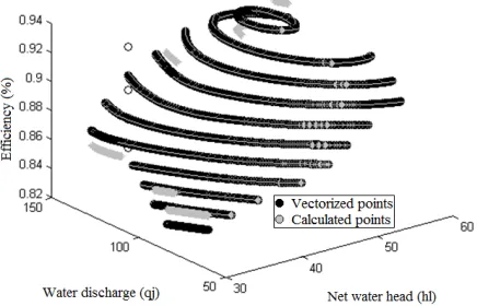
The existing relationship between generated power, net water head and water flow rate is usually represented by Hill Diagrams, given by turbine manufacturers for each specific unit [7]. For the studied plant, only a unique Hill Diagram characteristic exists for all the generation units. Then, the hydraulic loss model proposed in this work becomes very relevant. It allows for the calcula-tion of income-generating sets and to distinguish them from each other, since each machine will be uniquely characterized by a specific net hydraulic head. In order to find a good efficiency model for the plant, a non-linear multivariable regression process was performed. A Hill Diagram of the studied plant was digitized and vectorized. Also, a computer program was built to read the resulting digital image and convert each point of the original Hill Diagram in rectangular coordinates X, Y and Z, thus generating a vector of 6,969 points (hljt,
qjt,ηjt) relating power efficiency to the inflow rates and
net hydraulic heads of the generation units. As a result, Figure 1 presents the actual points generated by the Hill Diagram digitization process just described. The limits used to digitize, regarding the Hill Diagram for a Ka-plan type turbine, were:
• Indep. variable: water flow rate [50, 150] (m3/s); • Indep. variable: net hydraulic head [32, 56] (m);
• Dependent var.: global efficiency [83, 93] (%).
With these points in hand, a specific technique of nonlinear multivariable regression was implemented. This regression process was created using the statisti-cal toolbox of MATLAB cR2012b. This process uses the Levenberg-Marquardt algorithm [11] [13] to be per-formed. For the execution of this regression process, a subset of about 1,000 points arbitrarily chosen from the available set of 6,969 points, were used. Table 1
Figure 1:Hill Diagram resulted from digitization process
Table 1:Efficiency Coefficients obtained by the Regression Process
Coefficient Value
ρ0j 1.4630e-01
ρ1j 1.8076e-02
ρ2j 5.0502e-03
ρ3j -3.5254e-05
ρ4j -1.1234e-03
ρ5j -1.4507e-05
presents the coefficients obtained by the regression pro-cess, with 99% of accuracy.
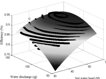
The validation of the coefficients shown in Table 1 and the resulting efficiency model represented by Eq. 7 can be seen in Figure 2, which shows the overlap of original (digitized) points and calculated (obtained through regression) points.
Figure 2:Original versus calculated points of the Hill Diagram
graph shows that the implemented regression process was satisfactory, as the coefficients estimated by non-linear multivariable regression provided a Hill Diagram very similar to the original one.
Figure 3:Generalization test for the adjusted model of the Hill Dia-gram
As shown by Eq. 7, power production function de-pends directly onqjtandhljt. But as the net hydraulic
headhljtcan be approximated by a function of the
wa-ter flow rateqjt, Finardi [7] proposed a simplified
pro-duction function as a polynomial of seventh degree in terms of coefficients associated withqjt, according to
Eq. 8. This function was also used in the model pro-posed by Araújo [2].
pjt(qjt) =ρ0jqjt+ρ1jq2jt+...+ρ6jqjt7. (8)
According to Finardi [7], coefficientsρ0j,...,ρ6jare
parameters dependent on operating characteristics and are calculated using the Hill Diagram, losses in pen-stocks and gross losses, among others. But using the efficiency model proposed by Finardi, only 6 operat-ing coefficients can be obtained, and his function uses 7 coefficients. Then, it becomes impossible to solve the problem, making use of this function, without further information about system conditions. Another relevant fact is that the author does not explain or justify the con-struction of his model. Given this modeling problem, this paper proposes a different function for calculating electric power, according to Eq. 9,
phjt=g·[ρ0j+ρ1jhljt+ρ2jqjt+ρ3jhljtqjt+ (9)
ρ4jhljt2 +ρ5jq2jt]·[Hbjt−∆Hjt]·qjt,
in which,
• phjtis the power generated by unitjat timet;
• g is the acceleration of gravity (9.8 ·
10−3kg/m2s2);
• ρ0j, ... ,ρ5j are the coefficients obtained from the
Hill Diagram using nonlinear multivariable regres-sion technique;
• hljtis the net hydraulic head of unitjat timet;
• qjtis the water flow rate of unitjat timet;
• ∆Hjtare the total losses referring to the penstock
connected to generation unitjat timet.
2.4 Optimization Model
According to the whole mathematical model presented so far, the goal of optimization is to maximize the hy-droelectric production function, taking into account all the generating units as represented by the objective function shown by Eq. 10. The vector optimization variables are represented by the water flow rate of each generation unit,
x= [q1t;q2t...qjt].
M aximize F(x) = PJ(r)
j=1 phjt
PJ(r)
j=1 qjt
, (10)
subject to:
J(r)
X
j=1
phjt∼=D,
qjtmin≤qjt≤qjtmax,
phminjk
∅j
X
k=1
Zjk≤phjt≤phmaxjk
∅j
X
k=1 Zjk,
Zjk∈ {0,1},
∅j
X
k=1
Zjk≤1.
represented by the inequality constraints of the objec-tive function.
The first constraint indicates that the power to be de-livered should be equal to the power requested by con-sumer electric demands; the National System Operator (ONS, from the Portuguese name “Operador Nacional do Sistema”), a government agency which operates the whole power production of Brazil, accepts an error rate of up to 0.5% above or below the demanded power. The second constraint states that the calculated flow rate must comply with the minimum and maximum capac-ity of each generation unit. The third constraint requires that the corresponding generated power complies with the minimum and maximum capacity of each genera-tion unit. At last, the fourth constraint insures that each generation unit maintains its operating zone, i.e., stays on or off during the whole production period.
To optimize the proposed objective function, this work proposes the use of GA, a sub-field of evolution-ary computation proposed by James Holland [10] in the seventies, in order to find optimal water flow rates for each generation unit and seeking to decrease the value of the optimization variables as low as possible, while maintaining the desired constraints still valid.
3 Optimization Algorithms
An algorithm is a sequence of executable actions to ob-tain a solution to a particular problem. In the context of Operational Research, algorithms are practical im-plementations of optimization methods, whose goal is to determine the solutions for a specific problem. This paper proposes the use of GA to solve the discussed op-timization problem (see Eq. 10).
3.1 Genetic Algorithms
GA are a metaheuristic technique used in computer sci-ence to find approximated solutions to optimization and search problems. GA are a particular class of evolu-tionary algorithms that use operations inspired by evo-lutionary biology such as inheritance, mutation, natu-ral selection and crossover [9]. GA are implemented as a computer program in which a population of ab-stract representations of solutions to a given problem is evolved in a search of better solutions. The evolution usually starts from a set of randomly created solutions and is carried through generations. At each generation, the adjustment of each individual (or solution) in the population is evaluated. Some individuals are selected for the next generation, and mutated or recombined to form a new population.
The new population is used as input for the next it-eration of the algorithm. This loop is executed until candidate solutions meet the expected outcome by the implemented fitness function. The binary representa-tion is the basic way to translate the actual problem in a viable way to be processed by the computer program. Importantly, the representation of a chromosome (or in-dividual) is critical to GA. The works [2], [3] and [15] reported that the use of GA gave satisfactory results for the problem of electric dispatch.
Considering those reports, this technique is applied as the main strategy to find good solutions for the prob-lem. Note that this problem is not simple to solve with conventional techniques. These algorithms are based on unrealistic assumptions of linearity and convexity, which cannot be assumed in the case of nonlinear prob-lems. This work implements two versions of GA: the first one uses binary representation of solutions as indi-viduals (called BGA) and other uses real representation of solutions as individuals (called RGA). Figure 4 ilus-trates the difference between both approaches.
Figure 4:Binary and real-valued approaches of GA
To solve the dispatch problem, GA algorithms cre-ate populations of wcre-ater flow rcre-ates, where each individ-ual represents a feasible water flow rate for each gen-eration unit in the power plant. The adopted stop crite-rion is the number of iterations. The “Canonical GA”, as proposed by Goldberg [8], was chosen to be imple-mented in both cases. The adopted fitness function is the objective function (see Eq. 10) with an additional penalty equal to 0.5. Details of each implemented ver-sion are depicted in the next sections.
3.1.1 BGA - Operators and Parameters
Table 2:Parameters used by GA
Parameter Value
Population size 50
Crossover probability 60%
Mutation probability 2%
Exchange bit probability 50%
Gamma adjustment function 1.8
Maximum number of generations 50
3.1.2 RGA - Operators and Parameters
The crossover operator implemented in RGA uses the Simulated Binary Crossover (SBX) algorithm, as pro-posed by [5]. SBX is designed respecting the properties of single crossing point, but by averaging the values of the individuals, it estimates the best cut-off point for each crossing. The mutation operator uses a function polynomial which defines the best gene to be mutated, as proposed also by [5]. Individuals are represented by 1x6 real valued vectors. RGA used the same parameters as the BGA algorithm (see Table 2).
4 Case Study
The case study of this paper is a hydroelectric plant installed in Brazil, with a nominal power production capacity of about 400M W. This section will discuss the general characteristics of this plant, which operates with 6 generation units, as well as the experiments per-formed to solve the electric unit dispatch problem, with the use of two GA methods, as discussed in the preced-ing sections.
To simulate the plant behaviour, the efficiency model used the same coefficients shown in Table 1. The inputs to the algorithm are an hourly power demand generation order to be delivered by the plant and the hydraulic head of the reservoirHb, at the time of
gener-ation. The value ofHb for the plant in question ranges
between 32 and 56m. All generation units are consid-ered as identical, so the Hill Diagram coefficients are the same. The facility has other constraints as water flow rates per unit qjt and generated power per unit
phjt, namely:
• qjtmust be in the range [70, 140]m3/s;
• phjtmust be in the range [35, 66]M W.
4.1 Practical Experiments
To validate the model proposed in this work, this sec-tion presents two experiments performed with param-eters above described. As a first experiment, a test of daily demand was executed to verify the behaviour of
GA algorithms while trying to meet the demand and to minimize generation units’ water flow rates. The second experiment tested the hourly demand situation, which checked evolution behaviour of the proposed al-gorithms while they were trying to meet the demand saving water discharge. After all, an statistical analy-sis was performed to objectively verify what is the best approach to solve the problem.
The algorithms here described were implemented using MATLAB cR2012b. The experiments were per-formed on a Intel Dual Core 2.1GHz processor ma-chine, with 3GB of RAM, running MS-Windows.
4.1.1 Experiment 1: Daily Demand
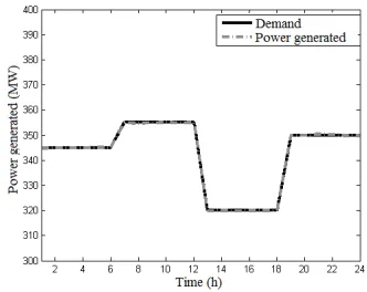
To demonstrate the feasibility of the solutions obtained by GA algorithms, when implemented as discussed in Section 3.1, an example of behaviour that shows a ran-dom daily demand follows. Simulations using all GA strategies have quite the same performance in terms of meeting the existing power constraints, as shown by fig-ures 5 and 6. This experiment used a hydraulic head of the reservoirHbof 54m.
Figure 5:Typical plot of power generated through time
As can be seen in Figure 5, the generated power demand and required power demand curves are over-lapped, certifying that the algorithm fulfilled the power production requirements. Moreover, it is clear in this experiment that the the total water discharge provided by the algorithm solution (identified by “determined by the algorithm” in the figure) was lower than the con-ventional solution (identified by “control mode” of op-eration in the figure), which corresponds to power de-mand equally distributed among the available genera-tion units. As shown by Figure 6, it is noticeable that the proposed “optimized mode” saves water during gen-eration, compared to the conventional “control mode”.
Figure 6:Typical plot of water flow rate through time
and 8. As can be seen, the algorithm respects the limits of power and water flow rates set by the system con-straints, because the values found for both, as for power as for water flow rates, are between the dotted lines, which represent in the graphics the respective limits of these variables.
Figure 7:Typical plot of power generated through time, per unit
This result shows that it is possible to optimize hy-droelectric operation applying different power demands for each generation unit inside a plant. It then con-tributes to the deconstruction of the hypothesis raised by [17], that “the optimal operating point of a hydro-electric plant is achieved only when the generation de-mand is equally divided by the number of generation units”.
4.1.2 Experiment 2: Hourly Demand
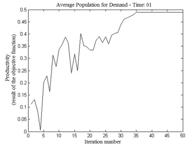
The main goal of this experiment is to find the aver-age processing time of each algorithm to achieve an optimized solution to dispatch problem. To check the behaviour of BGA and RGA algorithms, a demand of 320M Wwas established, since this is a typical demand of the plant. The hydraulic head of the reservoir, Hb,
was set to 54m. Figures 9 and 10 show plots of typical behaviour of the fitness functions for each algorithm,
Figure 8:Typical plot of water flow rate through time, per unit
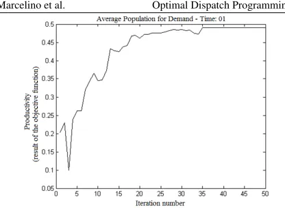
throughout generations, while they tried to maximize the plant productivity.
Figure 9:BGA - Evolution of fitness function through generations
It is clear from the figures that both algorithms con-verged to the best result since the 35th generation. One may notice that there is more sinuosity in BGA, which features higher falls than RGA. This means that for BGA it is harder to achieve stability. RGA presents lower sinuosity when compared to BGA. This fact in-dicates that RGA algorithm was able to obtain more confident results at each iteration, until reaching con-vergence at the35ageneration.
A typical simulation table report for BGA and RGA results is shown by Table 3. It presents the results for the best individual obtained by water flow rateqjtand,
through these values, other parameters are calculated from the mathematical model.
Figure 10:RGA - Evolution of fitness function through generations
Table 3:General Experiment Report
BGA |Hb= 54m
UN ph(M W) q(m3/s) η(%) hl(m) ∆ H(m)
1 49,719 101,41 0,93 53,796 0,20377
2 59,383 121,04 0,93 53,83 0,17007
3 62,218 126,81 0,93 53,833 0,16745
4 44,282 90,253 0,93 53,834 0,1656
5 57,078 116,33 0,93 53,834 0,1656
6 47,512 96,838 0,93 53,833 0,16745
SUM 320,19 652,68 Demand request: 320 (M W)
SUB 0,19 2,37 Mode S: 655,05 (m3/s)
RGA |Hb= 54m
UN ph(M W) q(m3/s) η(%) hl(m) ∆H(m)
1 51,047 104,14 0,93 53,785 0,21489
2 47,343 96,515 0,93 53,821 0,17935
3 58,589 119,44 0,93 53,823 0,17659
4 49,178 100,25 0,93 53,825 0,17464
5 60,31 122,94 0,93 53,825 0,17464
6 53,653 109,37 0,93 53,823 0,17659
SUM 320,12 652,65 Demand request: 320 (M W)
SUB 0,12 2,4 Mode SC: 655,05 (m3/s)
and consequently the highest rate of productivity, cor-responding to a water flow rate of 2.4m3/s. Expand-ing to one hour, this is equivalent to approximately 8.6 million litres of water. It is also easy to check that, in “optimized mode” of operation, all units reached maxi-mum efficiency of 93% with use of water flow rate de-termined by the algorithms.
4.2 Comparative Analysis of GA Algorithms
In order to ensure the central limit theorem of normal-ity, each execution of the algorithms was repeated for thirty times. Carrano [4] showed that evolutionary algo-rithms cannot be compared only by means of computa-tional performance. Being stochastic search heuristics,
it is feasible that each execution have a different result. With this in mind, a comprehensive analysis of the re-sults provided by GA approaches were developed and tested, by means of statistical inference and multiobjec-tive tools, as discussed in the following sections.
4.2.1 Tukey Test
To perform an objective analysis of the multiple ob-tained results sets, this study used analysis of vari-ance (ANOVA) by means of Tukey Test, to find rele-vant information that could differentiate the tested al-gorithms. This statistical method can be interpreted as a comparison between means of different groups of so-lutions and the variances of all individuals within those groups. Tukey’s strategy is to define the least signifi-cant difference between these means. The hypothesis to be considered in this test is the equality of results of the series of datasets provided by BGA and RGA algo-rithms, adopting a confidence interval of 95%. Table 4 shows the results of the performed Tukey Test. It indi-cates that the hypothesis of equality between means of factors it not rejected, because P-value is close to zero. In other words, this test indicated that the results of the compared algorithms did not have sufficient statistical evidence to be considered as different (better or worse) from each other.
Table 4:Tukey Test: BGA x RGA
Levels Center Min Max P-value
BGA-RGA 0.00053 0.00025 0.00816 0.00029
4.2.2 Multiobjective Analysis of a Mono-objective Problem
So far, this work approached the electric dispatch prob-lem in a mono-objective way. This section proposes an multiobjective (MO) analysis for this mono-objective problem, considering the value of the objective func-tion and the computafunc-tional time of each one of the al-gorithms as two new objectives to be simultaneously used while comparing them. Here, again, the execu-tions of each algorithm were repeated for thirty times, to achieve statistical validation of the experiments. To differentiate solutions obtained in an MO analysis, an approach quite widespread in the literature is the con-cept of “Pareto Dominance”.
1. The solutionxis at least equal toyfor all purposes; 2. The solutionxis greater thanyfor at least one goal.
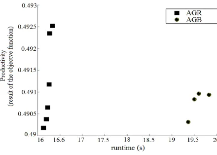
Thus, there is a set of solutions that have advantage over others, an optimal set of alternatives that are non-dominated by each other. The set of non-non-dominated so-lutions to a problem is usually called in the literature by a “Pareto Front”. For this analysis, a graphic was generated containing the Pareto Fronts obtained by both algorithms, as it is shown in Figure 11.
Figure 11:Comparative Pareto Front: BGA x RGA
It is noticeable from the graphic that the algorithm with the best Pareto Front is RGA, because its set of solutions has the lowest execution time, around 16.0s, and yet produced increasing values of power productiv-ity above 0.4925. It is also clear that the Pareto Front of RGA algorithm dominates the Pareto Front of BGA algorithm. From the MO point of view, considering av-erage execution time as a second goal,it can be stated that RGA performed better than BGA algorithm, while solving the electric dispatch problem in this experiment.
5 Conclusion
This paper proposed a novel mathematical modeling ap-proach to calculate hydraulic losses in penstocks at hy-droelectric plants, allowing for the calculation of elec-trical power production in a way distinct from previous works. This formulation was used inside an optimiza-tion schema to find optimal operating points for gen-eration units in an actual plant in Brazil. Given the discussed experimental results, it can be seen that op-timization methods based on Genetic Algorithms con-verged to satisfactory results.
Statistical analysis indicated that the approach using real representation of individuals (called RGA) showed better results than the approach using binary individu-als (called BGA) to solve the problem of electric
dis-patch. The productivity indexes found in “optimized mode”, using BGA and RGA, are higher than the value of the same index when running the plant in conven-tional “control mode”. This finding assures the rele-vance of the approach adopted in this work. Finally, the simplicity of the proposed model and the small amount of operational data necessary to implement it in prac-tice indicate that this approach can easily be applied to other case studies, what makes it fairly general.
Acknowledgement
The authors would like to thank CEMIG and Or-teng, for the cession of operational data and support, ANEEL and CEMIG for the grant GT333-2011, and CEFET-MG for the infrastructure used in this project.
References
[1] Almeida, P. E. M. Optimization of voltage and power ensemble control for electric energy gener-ation with use of artificial intelligence. Technical report, Annual Research & Development Program CEMIG/ANEEL - Cycle 2007/2008, 24p (in Por-tuguese), 2007.
[2] Araújo, R. Hydroelectric energy production modeling and optimization: an approach with the use of intelligent systems. Master’s thesis, CEFET-MG (in Portuguese), 2010.
[3] Baños, R. Optimization methods applied to re-newable and sustainable energy: a review. EL-SEVIER, In: Renewable and Sustainable Energy Reviews, 15:1753–1766, 2011.
[4] Carrano, E., Wanner, E., and Takahashi, R. A multicriteria statistical based comparison method-ology for evaluating evolutionary algorithms. IEEE Transactions on Evolutionary Computation, 15:848–870, 2010.
[5] Deb, K. and Agrawal, R. Simulated binary crossover for continuos search space. Convenor, Technical Reports, 34p, 1994.
[6] Dudek, G. Unit commitment by genetic algorithm with specialized search operators. ESELVIER In: Eletric Power Systems Research, 74:299–308, 2004.
[8] Goldberg, D. E. Genetic Algorithms in Search, Optimization and Machine Learning. Addison-Wesley, ISBN 978-0201157673, 1989.
[9] Goldberg, D. E., Harik, G., and Lobo, F. The com-pact genetic algorithm.IEEE Trans. on Evolution-ary Computation, 3(4):287–297, 1999.
[10] Holland, J. H. Adaptation in natural and artificial systems. Michigan Press, ISBN 978-0262581110, 1975.
[11] Levenberg, K. A method for the solution of certain non-linear problems in least squares.Quarterly of Applied Mathematics 2, pages 164–168, 1944.
[12] Marcelino., C. Optimization of a ensemble control system for hydroelectric energy generation with use of computational intelligence. Master’s thesis, CEFET-MG (in Portuguese), 2012.
[13] Marquardt, D. An algorithm for least-squares es-timation of nonlinear parameters. SIAM Journal on Applied Mathematics, 11(2):431–441, 1963.
[14] Netto, A. Hydraulics Manual. 8a Ed, Edgard Blucher, ISBN 978-8521202776 (in Portuguese), 1998.
[15] Pezzini, P. Optimization techniques to improve energy efficiency in power systems. ELSEVIER In: Renewable and Sustainable Energy Reviews, 15:2028–2041, 2011.
[16] Porto, R. Basic Hydraulics. EDUSP, São Paulo, ISBN 978-8576560845 (in Portuguese), 2004.
[17] Ribas, F. Optimization of energy generation in hy-droelectric plants. InTracbel 3oSEPOCH, Paraná
(in Portuguese), 2002.