www.theoryofcomputing.org
Improved Inapproximability for TSP
Michael Lampis
∗Received November 28, 2012; Revised November 27, 2013; Published September 27, 2014
Abstract: The Traveling Salesman Problem is one of the most studied problems in the theory of algorithms and its approximability is a long-standing open question. Prior to the present work, the best known inapproximability threshold was 220/219, due to Papadimitriou and Vempala. Here, using an essentially different construction and also relying on the work of Berman and Karpinski on bounded-occurrence CSPs, we give an alternative and simpler inapproximability proof which improves the bound to 185/184.
ACM Classification:G.1.6
AMS Classification:68Q17
Key words and phrases:inapproximability, traveling salesman
1
Introduction
The Traveling Salesman Problem (TSP) is one of the most widely studied algorithmic problems and deriving optimal inapproximability results for it is a long-standing question. On the algorithmic front, there has been much progress recently, at least in the important special case where the metric is derived from an unweighted graph. This case is often referred to as the Graphic TSP. For over 30 years, the 3/2-approximation algorithm by Christofides [5] (1976) was the best result known. This changed in 2011 when Gharan, Saberi, and Singh gave a slight improvement [8] for Graphic TSP. Subsequently an algorithm with approximation ratio 1.461 was given by Mömke and Svensson [13]. With improved analysis of their algorithm, Mucha obtained a ratio of 13/9 [14]. The best currently known algorithm has ratio 1.4 and is due to Seb˝o and Vygen [18].
A conference version of this paper appeared in the Proceedings of the 15th International Workshop on Approximation Algorithms for Combinatorial Optimization Problems (APPROX’2012) [12].
Nevertheless, there is still a significant gap between the guarantee of the best approximation algorithms we know and the best inapproximability results. The TSP was first shown to beNP-hard to approximate to within 1+ε, for someε>0 by Papadimitrious and Yannakakis [17] but no explicit inapproximability
constant was derived. The work of Engebretsen [6] and Böckenhauer et al. [4] gave inapproximability thresholds of 5381/5380 and 3813/3812, respectively. Later this was improved to 220/219 in [16] by Papadimitriou and Vempala.1 No further progress has been made on the inapproximability threshold of this problem in the more than ten years since the conference version of the Papadimitriou and Vempala paper appeared ([15]). For the special case of the problem with bounded metrics the works of Engebretsen and Karpinski [7] and more recently Karpinski and Schmied [11] give inapproximability constants only slightly weaker than those known for the general version.
Overview: Our main objective in this paper is to give a different, less complicated inapproximability proof for TSP than the one given in [15,16]. The proof of [16] is very much optimized to achieve a good constant: the authors reduce directly from MAX-E3-LIN2, a constraint satisfaction problem (CSP) where each constraint is a mod 2 linear equation in exactly 3 variables. For MAX-E3-LIN2, optimal inapproximability results are known, due to Håstad [9]. They take care to avoid introducing extra gadgets for the variables, using only gadgets that encode the equations. Finally they define their own custom expander-like notion on graphs to ensure consistency between tours and assignments. Then the reduction is performed in essentially one step.
Here on the other hand we take the opposite approach, choosing simplicity over optimization. We also start from MAX-E3-LIN2 but go through two intermediate CSPs. The first step in our reduction gives a set of equations where each variable appears at most five times (this property will come in handy in the end when proving consistency between tours and assignments). In this step, rather than introducing something new we rely heavily on machinery developed by Berman and Karpinski to prove inapproximability for bounded-occurrence CSPs [1,2,3]. As a second step we reduce to MAX-1-IN-3-SAT, a CSP where each constraint requires exactly one out of three literals to be true. The motivation is that the 1-IN-3 predicate nicely corresponds to the objectives of TSP, since we represent clauses by gadgets and the most economical solution will visit all gadgets once but not more than once. Another way to view this step is that we use MAX-1-IN-3-SATas an aid to design a TSP gadget for parity. Finally, we give a reduction from MAX-1-IN-3-SATto TSP.
This approach is (arguably) simpler than the approach of [16], since some of our arguments can be broken down into independent pieces, arguing about the inapproximability of intermediate, specially constructed CSPs. We also benefit from using the amplifier constructed in [3]. Interestingly, putting everything together we end up obtaining a slightly better constant than the one known prior to this work. Though we are still a long way from an optimal inapproximability result, our results indicate that there may still be hope for better bounds with existing tools. Exploring how far these techniques can take us with respect to TSP (and also its variants, see for example [11]) may thus be an interesting question.
The main result of this paper is given below. The result follows directly from the construction in
Section 4.1and Lemmata4.1and4.2.
Theorem 1.1. There is no polynomial-time(92.3/91.8−ε)-approximation algorithm forTSPfor any
ε>0unlessP=NP.
Let us also note that, since the conference version of this paper appeared, recent work ([10]) has pushed the idea of building a modular reduction further. In particular, this has resulted not only in a further improvement of the inapproximability constant for TSP (to 123/122), but also in an improvement of the constant for the asymmetric case of the problem (from the 117/116 bound given in [16] to 75/74).
2
Preliminaries
We will denote graphs byG(V,E). All graphs are assumed to be undirected, loop-less and edge-weighted, meaning that there is also a functionw:E→R+. In some cases we will allowEto be a multi-set, that is, we may allow parallel edges. In the case of a multi-setEthat contains several copies of some elements, when we write∑e∈Ew(e)we mean the sum that has one term for each copy. A (multi-)graph is Eulerian
if there exists a closed walk that visits all its vertices and uses each edge once. It is well known that a (multi-)graph is Eulerian iff it is connected and all its vertices have even degree. We will use[n]to denote the set{1,2, . . . ,n}. We will useE[X]to denote the expectation of a random variableX.
In the metric Traveling Salesman Problem (TSP) we are given as input an edge-weighted undirected graphG(V,E). Letd(u,v), foru,v∈V denote the shortest-path distance fromutov. The objective is to find an orderingv1,v2, . . . ,vnof the vertices such that∑ni=−11d(vi,vi+1) +d(vn,v1)is minimized. Note that this is equivalent to the alternative formulation of the problem where we are given all pairwise distances between points and distances satisfy the triangle inequality: shortest path distances on a graph always satisfy the triangle inequality, and the input graph is allowed to be an edge-weighted clique.
Another, equivalent view of the TSP is the following: given an edge-weighted graphG(V,E)we seek to find a multi-setET consisting of edges fromE such thatET spansV, the graphGT(V,ET)is
Eulerian and the sum of the weights of all edges inET is minimized. It is not hard to see that the two
formulations are equivalent. (The subscriptT refers to the Eulerian “tour.”) We will make use of this second formulation because it makes some arguments on our construction easier.
We generalize the Eulerian multi-graph formulation as follows. A multi-setET of edges fromE
is aquasi-tour if the degrees of all vertices in the multi-graph GT(V,ET) are even. In other words,
a quasi-tour is a tour that is not required to be connected. The cost of a quasi-tour is defined as
∑e∈ETw(e) +2(c(GT)−1), wherec(GT) denotes the number of connected components of the
multi-graph. The intuition is that we want to allow quasi-tours (because this will simplify some proofs) but penalize them for leaving some components disconnected. It is not hard to see that a TSP tour can also be considered a quasi-tour with the same cost (since for a normal tourc(GT) =1), but in a weighted
graph there could potentially be a quasi-tour that is cheaper than the optimal tour. One useful property of quasi-tours is the following:
Lemma 2.1. There exists a quasi-tour of minimum cost such that all edges with weight one are used at most once.
2.1 Forced edges
As mentioned above, we will view TSP as the problem of selecting edges fromEto form a minimum-weight multi-setET that makes the graph Eulerian. It is easy to see that no edge will be selected more
than twice, since if an edge is selected three times we can remove two copies of it fromET and the graph
will still be Eulerian while we have improved the cost.
In our construction we would like to be able to stipulate that some edges are to be used at least once in any valid tour. We can achieve this with the following trick. Suppose that there is an edge(u,v)with weightwthat we want to force into every tour. We sub-divide this edge a large number of times, say p−1 times, that is, we remove the edge and replace it with a path of pedges going through new vertices of degree two. We then distribute the original edge’s weight to thepnewly formed edges, so that each has weightw/p. Now, any tour that omits two or more of the newly formed edges must be disconnected. Any tour that omits exactly one of them can be augmented by adding two copies of the unused edge. This only increases the cost by 2w/p, which can be made arbitrarily small by givingpan appropriately large value. Therefore, we may assume without loss of generality that in our construction we can force some edges to be used at least once. Note that these arguments apply also to quasi-tours.
Another way to summarize the above is the following. Let F-TSP be the version of the problem where the input also contains forced edges. If F-TSP isNP-hard to approximate within some constant cthen for allε >0, TSP isNP-hard to approximate withinc−ε. In other words, the problems are
essentially equivalent, and because of this we will focus on the version of the problem where edges can be forced, and simply refer to it as TSP from now on.
3
Intermediate CSPs
In this section we will design a family of instances of MAX-1-IN-3-SATwith some special structure and prove their inapproximability. We will use these instances (and their structure) in the next section where we reduce from MAX-1-IN-3-SATto TSP.
LetI1be a system ofmlinear equations mod 2, each consisting of exactly three variables. Letnbe the total number of variables appearing inI1and let the variables be denoted asxi,i∈[n]. LetBbe the
maximum number of times any variable appears. We will make use of the following seminal result due to Håstad [9]:
Theorem 3.1(Håstad). For allε>0there exists an integer B such that given an instance I1as above it isNP-hard to distinguish the case when there is an assignment that satisfies at least(1−ε)m equations
from the case when all assignments satisfy at most(1/2+ε)m equations.
3.1 Bounded occurences
InI1each variable appears at mostBtimes, where the constantBdepends onε. We would like to reduce
Theorem 3.2(Theorem 3 in [3]). Let B be a multiple of 5. Then for all sufficiently large B there exists a bipartite graph G(L,R,E), with|L|=B,|R|=0.8B, all vertices of L having degree 4 and all vertices of R having degree 5 that additionally has the following connectivity property: for any S⊆L∪R such that
|S∩L| ≤ |L|/2the number of edges in E with exactly one endpoint in S is at least|S∩L|.
Unfortunately, a full version of [3] has not appeared so far. We therefore provide a (slightly simplified) proof ofTheorem 3.2below just for the sake of completeness. The reader may feel free to skip this proof as only the statement ofTheorem 3.2is needed for the rest of the paper.
Proof. The proof proceeds via the probabilistic method. Let L, Rbe two sets of vertices such that
|L|=|R|=4n, wherenis a multiple of 5. First, partitionLintonsets of size 4 andRinto 0.8nsets of size 5 each. Then, select a perfect matching fromLtoRuniformly at random. Collapse each set from the partitions ofL,Rinto a single vertex. It is easy to see that we have constructed a random bipartite graph that is 4-regular on one side and 5-regular on the other. We will show that with high probability the graph also satisfies the connectivity property. In particular, we will show that for someε>0 the probability
(over the random matchings) that there exists a “bad” setSviolating the property is at most 2−εn, which
tends to 0 for largen. More precisely, we will examine various “configurations” thatScan have, and find the configuration which has the maximum probability of being bad. We will then show that this is so small that by taking a union bound we can guarantee that with high probability no bad set exists.
If there exists such a bad setS, we can assume without loss of generality that vertices ofRbelong toS if and only if the majority of their neighbors are inS. In other words, all of the setScan be determined by S∩L, while the placement of vertices ofRintoSandV\Scan be done greedily by counting the number of neighbors each vertex has inS, because doing so can only decrease the size of the produced cut.
Suppose we have a setSsuch that|S∩L|=s. LetAi,i∈ {0,1, . . . ,5}be the set of vertices ofRthat
have exactlyineighbors inS. Thus,S= (S∩L)∪A5∪A4∪A3. We denote|Ai|=aiand let the number of
edges with exactly one endpoint inSbec. The probability that a specific subset ofLof sizeswill attain the configuration described (that is,aivertices ofRhaveineighbors inSandcedges are cut in total) can
be calculated exactly as:
P(n,s,c,ai) =
(0.8n)!
∏5i=0ai!
5a1+a410a2+a3(4s)!(4n−4s)!
(4n)! . (3.1)
Let us explain this. We count the number of matchings that lead to such a configuration. First, we can select a partition of the 0.8nvertices ofRinto the setsAi, so the first factor is an expansion of
0.8n a0,a1,a2,a3,a4
.
Of course, for the above calculation to make sense the numbersn,s,c,ai must obey some further
constraints. In particular:
a0+a1+a2+a3+a4+a5=0.8n, (3.2)
a1+2a2+2a3+a4=c, (3.3)
a1+2a2+3a3+4a4+5a5=4s, (3.4)
c<s≤0.5n. (3.5)
Constraint (3.2) simply states that theAipartitionR. Constraint (3.3) measures the number of cut
edges. Constraint (3.4) makes sure that a perfect matching is possible using the selected number of endpoints. Finally, constraint (3.5) states that we are interested in a bad set.
Since all subsets ofL of size s are equivalent, by union bound the probability that there exists a set of sizesachieving a certain configuration is at mostU(n,s,c,ai) =P(n,s,c,ai) ns
. Expanding equation (3.1) we get
U(n,s,c,ai) =
(0.8n)!
∏5i=0ai!
5a1+a410a2+a3(4s)!(4n−4s)!
(4n)!
n s
. (3.6)
Our proof strategy consists of showing that the maximum value ofU(n,s,c,ai)subject to constraints
(3.2), (3.3), (3.4), (3.5) is at most 2−εn. If we show this, because there are only polynomially (inn) many
choices for the parameterss,c,ai, again by union bound we will have shown that the probability that a
bad set exists tends to 0. Thus, the rest of the proof consists of finding the values that maximizeUas a function ofnand showing an upper bound on this maximum. We do this by proving a series of intuitive (though sometimes tedious) claims.
Before we go on, let us simplify the constraints slightly. From constraints (3.3) and (3.5) we have that a1+a2+a3+a4≤s, while from constraint (3.4) we have thata1+a2+a3+a4+5a5≤4s. Multiplying the first inequality with 4 and summing we get (after dividing by 5)a1+a2+a3+a4+a5≤1.6s. Using constraint (3.2) this gives
a0≥0.8n−1.6s. (3.7)
We will now find an upper bound on the maximum value attainable byUsubject to constraints (3.2), (3.3), (3.5), (3.7). Notice that we have added constraint (3.7), which was already implied by the other constraints, so this cannot affect the maximum, while we dropped constraint (3.4), which can only make the maximum larger.
Claim 3.3. The function U(n,s,c,ai)when subject to constraints(3.2),(3.3),(3.5)and(3.7)is maximized
when|n/2−s|=O(1).
Proof. Intuitively, this claim makes sense, since it states that bisections ofLare the most problematic case, as one would expect. Suppose we have some other configuration withssignificantly smaller than n/2. We will create a configuration wheresis closer ton/2 andUis increased as follows: decreasenby 5, decreasea0by 4 and leave all other parameters unchanged. Observe that all four constraints are still satisfied. NowUis multiplied by a factor of
a40
(0.8n)4 n15
Let us explain this. First, becauses is significantly smaller thann/2 by constraint (3.7) we know thata0is large, so the change due toa0can indeed be approximated bya40(instead of the more accurate a0(a0−1)(a0−2)(a0−3)). In addition, the exponent ofnis 15 (and not 20), becauseU also contains the nsfactor.
Since we only care about sufficiently largen, it is enough to show that the limit of this value is greater than 1, or equivalently thata0/(0.8n)>(1−s/n)3.75.
Observe that from constraints (3.2), (3.3) and (3.5) we can conclude thata0+a5≥0.3n. Also, if a5>a0, then we can subtract 1 froma5and add 1 toa1. In this case, none of the four constraints is violated andUincreases. Therefore, we can conclude thata0≥0.15n.
Now, let us distinguish two cases. Ifs/n≥0.4 then(1−s/n)3.75≤0.63.75≤0.148. Therefore in this case we havea0/(0.8n)≥0.15n/(0.8n) =0.1875>(1−s/n)3.75.
Ifs/n≤0.4 then we use the fact that(1−s/n)3.75is a convex function ofs. Fors=0 the function has of course value 1, while fors=0.4nit has value 0.63.75≤0.148<0.2. The value of a convex function f in an interval[a,b]is upper-bounded by the value of a linear function that coincides with f on pointsa andb. In this case we will overestimate the value of(1−s/n)3.75ats=0.4nby pretending that it is 0.2, so the linear function that we get is 1−2s/n. We thus get that(1−s/n)3.75≤1−2s/nfors/n∈[0,0.4]. Buta0/(0.8n)≥1−2s/nby constraint (3.7), and we are done.
Thanks to the above claim we can assume that essentiallys=n/2, which makes constraint (3.7) vacuous. We will thus find an upper bound forUsubject to constraints (3.2), (3.3) and (3.5).
Claim 3.4. The function U(n,s,c,ai)when subject to constraints(3.2),(3.3), and (3.5)is maximized
when|ai−a5−i| ≤1, for i∈ {0,1, . . . ,5}.
Proof. Suppose thatai≥a5−i+2. Then decreaseaiby 1 and increasea5−iby 1. This does not violate
any of the three constraints and it increasesU.
Claim 3.5. The function U(n,s,c,ai)when subject to constraints(3.2),(3.3), and (3.5)is maximized
when c=s−1.
Proof. Suppose thatc<s−1. First, observe that it cannot be the case thata0≤a1≤a2anda5≤a4≤a3, because thena0+a5<0.3nand constraint (3.5) will be violated. So suppose we havea0>a1(and the casesa1>a2,a5>a4anda4>a3are similar). Then decreasea0by 1, increasea1by 1 and increasec by 1. This increasesUwithout violating any constraint.
Our problem now becomes
maxU(n,s,c,ai) =
(0.8n)!
∏2i=0(ai!)2
52a1102a2(2n)!(2n)!
(4n)!
n! (n/2)!2
s.t.
a0+a1+a2=0.4n (3.8)
a1+2a2=0.25n (3.9)
We can use the new constraints to get a1=0.25n−2a2 and a0=0.15n+a2. We are trying to maximize the part ofUthat depends ona0,a1,a2, so we want to maximize
5a110a2 a0!a1!a2!
= 0.4
a2
(0.15n+a2)!(0.25n−2a2)!a2!
.
What is the value ofa2that maximizes the above quantity? Observe that if we increasea2by 1, the above quantity changes by a factor of
0.4(0.25n−2a2)2 a2(0.15n+a2)
(1±o(1)).
For the maximizing value ofa2this factor must tend to 1, so that neither increasing nor decreasinga2 by 1 can improveU. We therefore get 0.4(0.25n−2a2)2=a2(0.15n+a2). Solving this fora2we get eithera2≈0.04796n, or a root that is larger than 0.8n, which we can ignore. From the first root we get a0≈0.19796nanda1≈0.15407n.
We can now plug in the above values intoU. Using Stirling formula we can approximate log(n!)with nlog ne+o(n), so we get
logU=0.8nlog
0.8n e
−
2
∑
i=0 2ailog
a i
e
+2a1log 5+2a2log 10+4nlog
2n e
−4nlog
4n e
+nlogn e
−nlogn 2e
=0.8nlog 0.8−
2
∑
i=0 2ailog
ai
n
+2a1log 5+2a2log 10−3n<−0.045n.
Thus, for sufficiently largenthe probability that there exists a bad set is at most 2−0.045n+o(n), which tends to 0. This completes the proof ofTheorem 3.2.
We now use the above theorem to construct a system of equations where each variable appears exactly 5 times. Our technique is pretty standard (in fact, essentially identical arguments are used in [3]). First, we may assume that inI1the number of appearances of each variable is a multiple of 5 (otherwise, repeat all equations five times). Also, by repeating all the equations we can make sure that all variables appear at leastB0times, whereB0is a sufficiently large number to makeTheorem 3.2hold.
For each variablexiinI1we introduce the variablesx(i,j),j∈[d(i)]andy(i,j),j∈[0.8d(i)]whered(i) is the number of appearances ofxi in the original instance. We call
the cloud that corresponds toxi. We will also useMto denote the set of thex(i,j)variables, which we call main variables, andCto denote the set of they(i,j)variables, which we call checker variables. Construct a bipartite graph with the property described inTheorem 3.2withL= [d(i)],R= [0.8d(i)](sinced(i)is a constant that depends only onεthis can be done in constant time by brute force). For each edge(j,k)∈E
introduce the equationx(i,j)+y(i,k)=1. Finally, for each equationxi1+xi2+xi3 =binI1, where this is the j1-th appearance ofxi1, the j2-th appearance ofxi2 and the j3-th appearance ofxi3 replace it with the equationx(i1,j1)+x(i2,j2)+x(i3,j3)=b.
Denote this instance byI2. Since we started with an instance withmequations of size 3, we had in total 3mvariable appearances, each of which has been replaced by a new variablex(i,j). We have also introduced 0.8×3m=2.4mvariablesy(i,j). Eachx(i,j)variable will now appear in 4 equations of size 2 (because the bipartite amplifier is 4-regular on one side). Thus,|I2|has 5.4mvariables and 13mequations in total, with 12mof these equations having size 2. Let us note that this problem, where equations of different sizes are mixed, is called the Hybrid problem in the work of Berman and Karpinski [3]. A consistent assignment to a cloudZi is an assignment that sets allx(i,j)tob and ally(i,j) to 1−b. By standard arguments using the graph ofTheorem 3.2we can show that an optimal assignment toI2is consistent as follows: suppose that we have an inconsistent assignment for a cloudZi. Let
S0={x(i,j)|x(i,j)=0} ∪ {y(i,j)|y(i,j)=1}
and letS1=Zi\S0. In other words,S0contains the variables consistent with a 0 assignment to thex(i,j) variables andS1those consistent with a 1 assignment. Any size-two equation containing exactly one variable fromS0 and one fromS1is violated by this assignment. By the properties of the graph, the number of such equations is at least as large as the number ofx(i,j)vertices in eitherS0orS1. Thus, we can flip the assignment of all the variables in one of the two sets and not decrease the number of satisfied equations.
Summary: Let us now summarize the properties of the instanceI2we have constructed that we will need later.
• The variable set is partitioned into the setM of main variables x(i,j) and the setC of checker variablesy(i,j). We have|M|=3m,|C|=2.4m.
• Each variable appears five times.
• There aremequations of size three and 12mequations of size two.
• The 12mequations of size two can be partitioned inton“clouds.” Each cloud consists of equations of the formx(i,j)+y(i,j0)=1.
• There is an optimal assignment that satisfies all equations of size two.
Theorem 3.6. Given aMAX-LIN2instance I2as above, for allε>0it isNP-hard to distinguish whether
3.2 MAX-1-IN-3-SAT
In the MAX-1-IN-3-SATproblem we are given a collection of clauses(`i∨`j∨`k), each consisting of at
most three literals, where each literal is either a variable or its negation. A clause is satisfied by a truth assignment if exactly one of its literals is set to True. The problem is to find an assignment that satisfies the maximum number of clauses.
We would like to produce a MAX-1-IN-3-SATinstance fromI2. Observe that it is easy to turn the size two equationsx(i,j)+y(i,k)=1 to the equivalent clauses(x(i,j)∨y(i,k)). We only need to worry about themequations of size three.
If thek-th size-three equation ofI2isx(i1,j1)+x(i2,j2)+x(i3,j3)=1 we introduce three new auxiliary variablesa(k,i),i∈[3]and replace the equation with the three clauses
(x(i1,j1)∨a(k,1)∨a(k,2)), (x(i2,j2)∨a(k,2)∨a(k,3)), (x(i3,j3)∨a(k,1)∨a(k,3)).
If the right-hand-side of the equation is 0 then we add the same three clauses except we negatex(i1,j1)in the first clause. We call these three clauses the cluster that corresponds to thek-th equation.
It is not hard to see that if we fix an assignment tox(i1,j1),x(i2,j2),x(i3,j3)that satisfies thek-th equation ofI2 then there exists an assignment to a(k,1),a(k,2),a(k,3) that satisfies the whole cluster. Otherwise, at most two of the clauses of the cluster can be satisfied. Furthermore, in this case there exist three different assignments to the auxiliary variables that satisfy two clauses and each leaves a different clause unsatisfied.
We will denote byAthe set of (auxiliary) variablesa(k,i). Call the instance of MAX-1-IN-3-SATwe have constructedI3. Note that it consists of 15mclauses: the 12mequations of size two fromI2give 12mclauses, while themequations of size three give 3 clauses each. The new instanceI3contains 8.4m variables: the 5.4mvariables ofI2plus 3 new auxiliary variables for each size-three equation ofI2.
Summary: Let us now summarize the properties of the instanceI3we have constructed that we will need later.
• The variable set is partitioned into the setMof main variablesx(i,j), the setCof checker variables y(i,j)and the setAof auxiliary variablesa(k,i). We have|M|=3m,|C|=2.4mand|A|=3m. • Each variable ofAappears twice. Each variable ofM∪Cappears five times. Each variable appears
negated at most once.
• There are 3mclauses of size three and 12mclauses of size two.
• The 3mclauses of size three can be partitioned intom“clusters.” Each cluster consists of three clauses of the form
(x(i1,j1)∨a(k,1)∨a(k,2)), (x(i2,j2)∨a(k,2)∨a(k,3)), (x(i3,j3)∨a(k,1)∨a(k,3)), with the possibility that the first literal of the first of these clauses may be negated.
• There is an optimal assignment that satisfies all clauses of size two.
Theorem 3.7. Given aMAX-1-IN-3-SATinstance I3as above, for allε>0it isNP-hard to distinguish if the maximum number of satisfiable clauses is at least(15−ε)m or at most(14.5+ε)m.
4
TSP
4.1 Construction
We now describe a construction that encodesI3into a TSP instanceG(V,E). Rather than viewing this as a generic construction from MAX-1-IN-3-SATto TSP, we will at times need to use facts that stem from the special structure ofI3, as summarized at the end of the previous section.
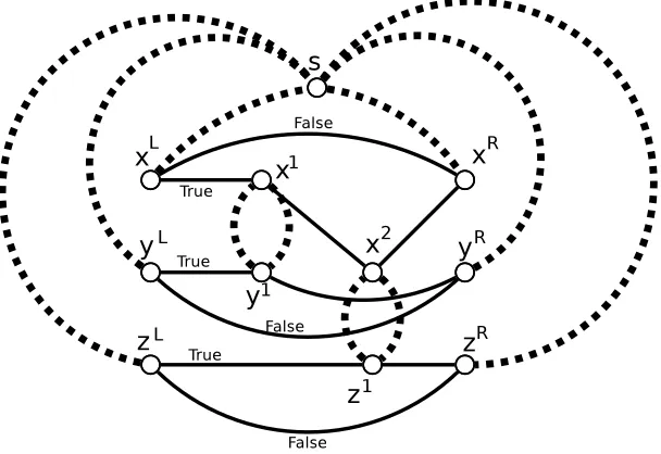
As mentioned, we assume that in the graphG(V,E)we may include some forced edges, that is, edges that have to be used at least once in any tour. The graph includes a central vertex, which we will calls. For each variable inx∈M∪C∪Awe introduce two new vertices namedxLandxR, which we will call the left and right terminal associated withx. We add a forced edge from each terminal tos. For terminals that correspond to variables inM∪Cthis edge has weight 7/4, while for variables inAit has weight 1/2. We also add two (parallel) non-forced edges between each pair of terminals representing the same variable, each having a weight of 1 (we will later break down at least one from each pair of these, so the graph we will obtain in the end will be simple, that is, it will not have parallel edges). Informally, these two edges encode an assignment to each variable: we arbitrarily label one the True edge and the other the False edge, the idea being that a tour should pick exactly one of these for each variable and that will give us an assignment. We will re-route these edges through the clause gadgets as we introduce them, depending on whether each variable appears in a clause positive or negative.
Now, we add some gadgets to encode the size-two clauses ofI3. The intuition here, which will also apply to size-three clause gadgets, is that we construct a vertex for each appearance of a literal in a clause and use forced edges to turn the vertices from the same clause into a connected component. Then, it will be most economical for the tour to visit each such component exactly once, thus simulating the 1-in-3 predicate. Let us now give more details.
Let(x(i,j1)∨y(i,j2))be a clause ofI3and suppose that this is thek1-th clause that containsx(i,j1)and the k2-th clause that containsy(i,j2),k1,k2∈[5]. Then we add two new vertices to the graph, call themx
k1 (i,j1) andyk2
(i,j2). Add two forced edges between them, each of weight 3/2 (recall that forced edges represent long paths, so these are not really parallel edges). Finally, re-route the True edges incident onxL(i,j
1)and yL(i,j
2)throughx
k1
(i,j1)andy
k2
(i,j2)respectively. More precisely, if the True edge incident onx
L
(i,j1)connects it to some other vertexu, remove that edge from the graph and add an edge fromxL(i,j
1)tox
k1
(i,j1)and an edge fromxk1
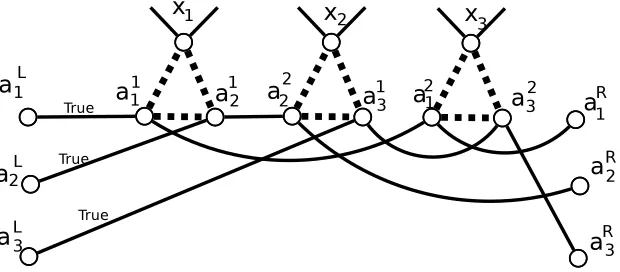
(i,j1)tou. All these edges have weight one and are non-forced (seeFigure 1). We use a similar gadget for clauses of size three (seeFigure 2). Consider a cluster
(x(i1,j1)∨a(k,1)∨a(k,2)), (x(i2,j2)∨a(k,2)∨a(k,3)), (x(i3,j3)∨a(k,1)∨a(k,3)),
and suppose for simplicity that this is the fifth appearance for all the main variables of the cluster. Then we add the new verticesx(5i
1,j1),x 5 (i2,j2),x
5
(i3,j3)and also the verticesa 1
Figure 1: Example construction for the clause(x∨y)∧(x∨z). Forced edges are denoted by dashed lines. There are two terminals for each variable and two gadgets that represent the two clauses. The True edges incident on the terminals are re-routed through the gadgets where each variable appears positive. The False edges connect the terminals directly since no variable appears anywhere negated. Forced edges incident onshave weight 7/4. All other forced edge in this figure have weight 3/2. All non-forced edges have weight 1.
To encode the first clause we add two forced edges of weight 5/4, one fromx5(i
1,j1)toa 1
(k,1)and one from x5(i
1,j1)toa 1
(k,2). We also add a forced edge of weight 1 froma 1 (k,1)toa
1
(k,2), thus making a triangle with the forced edges (seeFigure 2). We re-route the True edge fromaL(k,1)througha(1k,1)anda2(k,1). We do similarly for the other two auxiliary variables and the main variables. Finally, for a cluster wherex(i1,j1) is negated, we use the same construction except that rather than re-routing the True edge that is incident onxL(i
1,j1)we re-route the False edge. This completes the construction.
4.2 From assignment to tour
Let us now prove one direction of the reduction and in the process also give some intuition about the construction. Call the graph we have constructedG(V,E).
Lemma 4.1. If there exists an assignment to the variables of I3that leaves at most k equations unsatisfied, then there is a tour of G with cost at most T =L+k, where L=91.8m.
Figure 2: Example construction fragment for the cluster(x1∨a1∨a2)∧(x2∨a2∨a3)∧(x3∨a1∨a3). The False edges which connect each pair of terminals and the forced edges that connect terminals tosare not shown. The forced edges connectingaijtoxk have weight 5/4, while the third forced edge of each
triangle has weight 1.
in two clauses. Thus, we may assume that all clauses have a True literal. Also, we may assume that no clause has all literals set to True: suppose that a clause does, then both auxiliary variables of the clause are True. We set them both to False, gaining one clause. If this causes the two other clauses of the cluster to become unsatisfied, set the remaining auxiliary variable to True. We conclude that all clauses have either one or two True literals.
Our tour uses all forced edges exactly once. For each variablexset to True in the assignment the tour selects the True edge incident on the terminal corresponding tox. If the edge has been re-routed all its pieces are selected, so that we have selected edges that make up a path fromxLtoxR. Otherwise, ifxis set to False in the assignment the tour selects the corresponding False path.
Observe that this is a valid quasi-tour because all vertices have even degree (for each terminal we have selected the forced edge plus one more edge, for gadget vertices we have selected the two forced edges and possibly the two edges through which True or False was re-routed). Also, observe that the tour must be connected, because each clause contains a True literal, therefore for each gadget two of its external edges have been selected and they are part of a path that leads to the terminals.
The cost of the tour is at mostF+N+M+k, whereFis the total cost of all forced edges in the graph andN,Mare the total number of variables and clauses respectively inI3. To see this, notice that there are 2Nterminals, and there is one edge incident on each and there areMclause gadgets,M−kof which have two selected edges incident on them andkof which have four. Summing up, this gives 2N+2M+2k, but then each unit-weight edge has been counted twice, meaning that the non-forced edges have a total cost ofN+M+k.
4.3 From tour to assignment
We would like now to prove the converse ofLemma 4.1, namely that if a tour of costL+kexists then we can find an assignment that leaves at mostkclauses unsatisfied. Let us first give some high-level intuition and in the process justify the weights we have selected in our construction.
Informally, we could start from a simple base case: suppose that we have a tour such that all edges of Gare used at most once. It is not hard to see that this then corresponds to an assignment, as in the proof ofLemma 4.1. So, the problem is how to avoid tours that may use some edges twice.
To this end, we first give some local improvement arguments that make sure that the number of problematic edges, which are used twice, is limited. However, arguments like these can only take us so far, and we would like to avoid having too much case analysis.
We therefore try to isolate the problem. For variables inM∪Cwhich the tour treats honestly, that is, variables which do not appear in clauses whose corresponding gadgets have edges used twice, we directly obtain an assignment from the tour. For the other variables inM∪Cwe pick a random value and then extend the whole assignment toAin an optimal way. We want to show that the expected number of unsatisfied clauses is at mostk.
The first point here is that if a clause containing only honest variables turns out to be violated, the tour must also be paying an extra cost for it. The difficulty is therefore concentrated on clauses with dishonest variables.
By using some edges twice the tour is paying some cost on top of what is accounted for inL. We would like to show that this extra cost is larger than the number of clauses violated by the assignment. It is helpful to think here that it is sufficient to show that the tour pays an additional cost of 5/2 for each dishonest variable. This cost is enough since main and checker variables appear 5 times. By setting dishonest variables randomly we will satisfy half the clauses that contain them in expectation: clauses of size two are satisfied with probability 1/2 if at least one of their variables is randomly set, while for clauses of size three we assign the auxiliary variablesafterrandomly assigning the main variables, thus a whole cluster is satisfied if and only if the parity equation from which it was derived is satisfied and this happens with probability 1/2.
A crucial point now is that, by a simple parity argument, there has to be an even number of violations (that is, edges used twice) for each variable (Lemma 4.4). This explains the weights we have picked for the forced edges in size-three gadgets (5/4) and for edges connecting terminals tos(7/4=5/4+1/2 or 5/4 extra to the cost already included inLfor fixing the parity of the terminal vertex). Two such violations give enough extra cost to pay for the expected number of unsatisfied clauses containing the variable.
Let us now proceed to give the full details of the proof. Recall that if a tour of a certain cost exists, then there exists also a quasi-tour of the same cost. It suffices then to prove the following:
Lemma 4.2. If there exists a quasi-tour of G with cost at most L+k then there exists an assignment to the variables of I3that leaves at most k clauses unsatisfied.
In order to proveLemma 4.2it is helpful to first make some easy observations. First, recallLemma 2.1, which states that in an optimal quasi-tour all unit-weight edges are used at most once. All non-forced edges in our construction have unit weight and are therefore used at most once.
Second, if both forced edges of a gadget of size two are used twice then we can remove one appearance of each from the solution, decreasing the cost. Similarly, in a gadget of size three if two forced edges are used twice then we can drop one copy of each and use the third edge twice, making the tour cheaper. Therefore, in each gadget there is at most one forced edge that is used twice.
Third, if both forced edges that connect the terminalsxL,xRtosare used twice, then we can remove one appearance of each from the solution and replace them by the shortest path fromxLtoxRthat uses only non-forced unit weight edges. This has weight at most one for the auxiliary variables and two for the rest (since no variable appears negated more than once), which in both cases is at most as much as the weight of the removed edges. Therefore, for each variablex, at least one of the forced edges that connect xL,xRtosis used exactly once.
Given a tourET, we will say that a variablexis honestly traversed in that tour if all the forced edges
that involve it are used exactly once (this includes the forced edges incident onxL,xRandxi,i∈[5]). Let us now give two more useful facts.
Lemma 4.3. There exists an optimal tour where all forced edges between two different vertices that correspond to two variables in A are used exactly once.
Proof. We refer the reader again toFigure 2. Suppose we have an optimal tour that does not satisfy this property. We will transform it into a tour of the same or lower cost that does. Assume that the edge (a11,a12)is used twice (the other cases are equivalent by symmetry since all verticesaijare connected to one terminal and one other such vertex).
First, suppose that at least one of the edges that connect one of these two endpoints to a terminal is selected, say the edge(aL1,a11). Then modify the solution by removing that edge and a copy of the duplicate forced edge and adding a copy of(aL2,a12),(s,aL2)and(s,aL1). This does not increase the cost.
Second, suppose that both(s,aL1)and(s,aL2)are used twice in the tour. Then we can modify the tour by dropping one copy of each and a copy of the duplicate gadget edge and adding(aL1,a11)and(aL2,a12).
Finally, suppose that none of the previous two cases is true. Thus, neither of(aL1,a11),(aL2,a12)is used in the tour. This means that(a11,a21)and(a21,a22)are both used to ensure thata11anda12have even degree. Also, one of the edges connecting a terminal tosis used once, say(s,aL1). This means that the False edge incident toaL1 must be used to make the degree ofaL1even. Remove the False edge and the edge(a11,a21) from the tour and add the edges(aL1,a11)and(aR1,a21). This reduces to the first case.
Proof. Consider a variablexand first suppose that neither of the forced edges connectingsto the terminals is used twice, but there is a single forced edge in a gadget that is used twice. It follows that the vertex that corresponds toxin that gadget has an odd number of unit-weight edges incident to it selected. The two terminals have a single selected unit-weight edge incident on them and all other vertices that belong toxhave an even number of incident unit-weight edges selected, since their total degree is even. Thus, summing the number of selected unit-weight edges incident on all the vertices that belong toxwe get an odd number, which is a contradiction since we counted each such edge exactly twice. A similar argument applies if one assumes that one of the forced edges incident on the terminals is used twice and all other forced edges are used once.
Observe that it follows from Lemmata4.3and4.4that if all the main variables involved in a cluster are honest then the auxiliary variables of that cluster are also honest. This holds because if the main variables are honest then byLemma 4.3no forced edge inside the gadgets of the cluster is used twice, so byLemma 4.4and the fact that at least one of the forced edges incident on the terminals is used once, the auxiliary variables are honest.
We would like now to be able to extract a good assignment even if a tour is not honest, thus indirectly proving that honest tours are optimal.
Proof ofLemma 4.2. Consider the following algorithm to extract an assignment from the tour: first, for each variable inM∪Cthat was traversed honestly give it the same truth-value as in the tour, that is, if the tour selects the True edge incident on the corresponding terminal, set the variable to True, otherwise to False. To decide on the value of the dishonest variables fromM∪Cproducenrandom bitsbi,i∈[n]
(recall thatnis the number of variables ofI1, or the number of clouds inI2). For eachiset all dishonest variablesx(i,j)to be equal tobi and all dishonesty(i,j)to be equal to 1−bi. This ensures that size-two
clauses that contain two dishonest variables are always satisfied, since these clauses are always between two variables of the same cloud.
Let us also assign the auxiliary variables. If there is an assignment to the auxiliary variables of a cluster that satisfies all three clauses select it. Otherwise, select an assignment that violates the clause of a dishonest variable fromM, if such a variable exists, and satisfies the other two. If all main variables are honest, as we have argued the auxiliary variables are also honest, so pick the corresponding assignment.
We now have a randomized assignment forI3, so let us upper-bound the expected number of unsatisfied clauses. LetU be a random variable equal to the set of unsatisfied clauses and letU=U1∪U2whereU1 contains all the unsatisfied clauses that involve only honest variables fromM∪CandU2the rest. (Note thatU1is not random.)
The costT of the quasi-tour we have is≤F+N+M+k, where we remind the reader thatFis the cost of forced edges,Nis the number of variables ofI3andMthe number of clauses. LetEGbe the set of
forced gadget edges that the tour uses twice (each of these is included once inEG). LetESbe the set of
We have
T=
∑
e∈ET
w(e) +2(c(GT)−1) =F+
∑
e∈E1w(e) +
∑
e∈EG
w(e) +
∑
e∈ES
w(e) +2(c(GT)−1).
By definition∑e∈E1w(e) =|E1|. Let us try to lower-bound this quantity using arguments similar to the proof ofLemma 4.1. After the selection of the forced edges there are 2N− |ES|terminals with odd
degree, so each has a selected unit-weight edge incident to it. There are|U10|gadgets with at least four selected incident edges andM− |U10| − |U100|gadgets with two selected incident edges. Summing up we get 2N− |ES|+2M+2|U10| −2|U100|, but each edge is counted twice, so we have
|E1| ≥N− 1
2|ES|+M+|U
0
1| − |U
00
1|. Using this fact we get
T ≥F+N+M+
∑
e∈EG
w(e) +
∑
e∈ES
w(e)−1
2
+|U10|+2(c(GT)−1)− |U100|.
Now, observe that|U100| ≤c(GT)−1, because each element ofU100forms a component and there is
one component that is not an element ofU100(the one that containss). Thus, 2(c(GT)−1)− |U100| ≥ |U100|.
Combining this with the above we get
T ≥F+N+M+
∑
e∈EG
w(e) +
∑
e∈ES
w(e)−1
2
+|U10|+|U100|.
Given the known upper-bound on the cost of the tour we have that
k≥
∑
e∈EG
w(e) +
∑
e∈ES
w(e)−1
2
+|U10|+|U100|.
We now need to argue two facts and we are done. First|U1| ≤ |U10|+|U100|. Recall thatU1 is the set of unsatisfied clauses that involve honest variables. Since the variables are traversed honestly their corresponding gadgets are either visited at least twice or not at all, so they are counted in|U10|or in|U100|.
Second, we would like to show that
E[|U2|]≤
∑
e∈EG
w(e) +
∑
e∈ES
w(e)−1
2
.
Before we do that, observe that if we show this then it follows thatE[|U|] =E[|U2|] +|U1| ≤k, so there must exist an assignment that leaves no more thankclauses unsatisfied and we are done.
Let us define a credit cr(x)for each dishonest main or checker variablex. If a forced edge connecting a terminal tosis used twice we givexa credit of 5/4 (which is equal tow(e)−1/2, since these edges have weight 7/4). If a forced edge in a gadget that involvesxand another main or checker variable is used twice we givexa credit of 3/4 (which is equal tow(e)/2). Finally, if a forced edge in a gadget that involvesxand an auxiliary variable is used twice we givexa credit of 5/4 (which is equal tow(e)). We define cr(x)to be the sum of credits given toxin this process.
IfD⊆M∪Cis the set of dishonest main and checker variables then it is not hard to see that
∑
x∈D
cr(x)≤
∑
e∈EG
w(e) +
∑
e∈ES
(w(e)−1/2).
All edges are counted once in the sum of credits, except for those fromEGthat involve two main variables,
for which each is credited half the weight.
We will now argue that the expected number of unsatisfied clauses that contain a variablexis at most cr(x). Recall that clauses containingxand another dishonest main or checker variable are by construction satisfied, while clauses made up ofxand one honest variable are satisfied with probability 1/2. Also, clauses of size 3 that containxare satisfied with probability at least 1/2, since with probability 1/2 the equation from which the cluster was obtained is satisfied. Thus, if cr(x)≥5/2 we are done, becausex appears in 5 clauses and by the random assignment we will in expectation satisfy at least 5/2 clauses. We know thatxreceived at least two credits byLemma 4.4, so cr(x)≥3/2, as the smallest credit is 3/4. If cr(x) =3/2 thenx must have received two credits that were shared with other dishonest variables. Therefore, there are two clauses containingxwhich are surely satisfied, and out of the other three the expected number of unsatisfied clauses is 3/2≤cr(x). Similarly, if cr(x) =2, thenxshared a credit with another variable at least once, so one clause is surely satisfied and the expected number of unsatisfied clauses out of the other four is 2.
We therefore have
E[|U2|]≤
∑
x∈D
cr(x)≤
∑
e∈EG
w(e) +
∑
e∈ES
(w(e)−1/2) and this concludes the proof.
5
Conclusions
We have given an alternative and (we believe) simpler inapproximability proof for TSP, also modestly improving the known bound. We believe that the approach followed here where the hardness proof goes explicitly through bounded-occurrence CSPs, is more promising than the somewhat ad-hoc method of [16], not only because it is easier to understand but also because we stand to gain almost “automatically” from improvements in our understanding of the inapproximability of bounded-occurrence CSPs. In particular, though we used the 5-regular amplifiers from [3], any such amplifier would work essentially “out of the box,” and any improved construction could imply an improvement in our bound. In fact, in recent work [10] the hardness bound for TSP has been further improved, in part by substituting the 5-regular amplifiers with a new 3-regular amplifier construction.
References
[1] PIOTRBERMAN ANDMAREKKARPINSKI: On some tighter inapproximability results (extended abstract). InProc. 26th Internat. Colloq. on Automata, Languages and Programming (ICALP’99), volume 1644 ofLNCS, pp. 200–209. Springer, 1999. [doi:10.1007/3-540-48523-6_17] 218,220
[2] PIOTRBERMAN ANDMAREKKARPINSKI: Efficient amplifiers and bounded degree optimization. Electron. Colloq. on Comput. Complexity (ECCC), 8(53), 2001. ECCC. 218,220
[3] PIOTR BERMAN AND MAREK KARPINSKI: Improved approximation lower bounds on small occurrence optimization. Electron. Colloq. on Comput. Complexity (ECCC), 10(8), 2003. ECCC.
218,220,221,224,225,234
[4] HANS-JOACHIMBÖCKENHAUER, JURAJHROMKOVI ˇC, RALFKLASING, SEBASTIANSEIBERT, AND WALTER UNGER: An improved lower bound on the approximability of metric TSP and approximation algorithms for the TSP with sharpened triangle inequality. InProc. 17th Ann. Symp. on Theoretical Aspects of Comp. Sci. (STACS’00), volume 1770 ofLNCS, pp. 382–394. Springer, 2000. [doi:10.1007/3-540-46541-3_32] 218
[5] NICOSCHRISTOFIDES: Worst-case analysis of a new heuristic for the travelling salesman problem. Technical report, Carnegie-Mellon University, 1976. 217
[6] LARSENGEBRETSEN: An explicit lower bound for TSP with distances one and two.Algorithmica, 35(4):301–319, 2003. Preliminary version inSTACS’99. [doi:10.1007/s00453-002-1001-6] 218
[7] LARSENGEBRETSEN ANDMAREKKARPINSKI: TSP with bounded metrics.J. Comput. System Sci., 72(4):509–546, 2006. Preliminary version inICALP’01. [doi:10.1016/j.jcss.2005.12.001] 218
[8] SHAYANOVEISGHARAN, AMINSABERI,AND MOHITSINGH: A randomized rounding approach to the traveling salesman problem. InProc. 52nd FOCS, pp. 550–559. IEEE Comp. Soc. Press, 2011. [doi:10.1109/FOCS.2011.80] 217
[9] JOHANHÅSTAD: Some optimal inapproximability results. J. ACM, 48(4):798–859, 2001. Prelimi-nary version inSTOC’97. [doi:10.1145/502090.502098] 218,220
[10] MAREK KARPINSKI, MICHAEL LAMPIS, AND RICHARD SCHMIED: New inapproximability bounds for TSP. InProc. 24th Internat. Symp. on Symbolic and Algebraic Computation (ISAAC’13), volume 8283 ofLNCS, pp. 568–578. Springer, 2013. See also atECCC. [ doi:10.1007/978-3-642-45030-3_53] 219,234
[11] MAREKKARPINSKI AND RICHARD SCHMIED: On approximation lower bounds for TSP with bounded metrics. Electron. Colloq. on Comput. Complexity (ECCC), 19(8), 2012.ECCC. See also atarXiv. 218
ofLNCS, pp. 243–253. Springer, 2012. See also atarXiv. [doi:10.1007/978-3-642-32512-0_21]
217
[13] TOBIAS MÖMKE ANDOLASVENSSON: Approximating graphic TSP by matchings. Technical report, 2011. Preliminary version inFOCS’11. [arXiv:1104.3090] 217
[14] MARCINMUCHA: 139-approximation for graphic TSP.Theory Comput. Syst., 2012. Preliminary version inSTACS’12. [doi:10.1007/s00224-012-9439-7] 217
[15] CHRISTOSH. PAPADIMITRIOU ANDSANTOSHVEMPALA: On the approximability of the traveling salesman problem (extended abstract). In Proc. 32nd STOC, pp. 126–133. ACM Press, 2000. [doi:10.1145/335305.335320] 218
[16] CHRISTOSH. PAPADIMITRIOU ANDSANTOSHVEMPALA: On the approximability of the traveling salesman problem. Combinatorica, 26(1):101–120, 2006. Preliminary version in STOC’00. [doi:10.1007/s00493-006-0008-z] 218,219,234
[17] CHRISTOSH. PAPADIMITRIOU ANDMIHALISYANNAKAKIS: The traveling salesman problem with distances one and two. Math. Oper. Res., 18(1):1–11, 1993. [doi:10.1287/moor.18.1.1] 218
[18] ANDRÁSSEB ˝O ANDJENS VYGEN: Shorter tours by nicer ears: 7/5-approximation for graphic TSP, 3/2 for the path version, and 4/3 for two-edge-connected subgraphs. Technical report, 2012. To appear in Combinatorica. [arXiv:1201.1870] 217
AUTHOR
Michael Lampis
KTH Royal Institute of Technology mlampis kth se
http://www.csc.kth.se/~mlampis
ABOUT THE AUTHOR