http://theoryofcomputing.org
Near-Optimal Network Design
with Selfish Agents
∗
Elliot Anshelevich
†Anirban Dasgupta
‡Eva Tardos
´
§Tom Wexler
¶Received: September 26, 2007; published: August 4, 2008.
Abstract: We introduce a simple network design game that models how independent self-ish agents can build or maintain a large network. In our game every agent has a specific connectivity requirement, i. e. each agent has a set of terminals and wants to build a net-work in which his terminals are connected. Possible edges in the netnet-work have costs and each agent’s goal is to pay as little as possible. Determining whether or not a Nash equi-librium exists in this game is NP-complete. However, when the goal of each player is to connect a terminal to a common source, we prove that there is a Nash equilibrium on the optimal network, and give a polynomial time algorithm to find a(1+ε)-approximate Nash
equilibrium on a nearly optimal network. Similarly, for the general connection game we prove that there is a 3-approximate Nash equilibrium on the optimal network, and give an algorithm to find a(4.65+ε)-approximate Nash equilibrium on a network that is close to
optimal.
ACM Classification: G.2.2, F.2.2, F.2.3, J.4
AMS Classification: 68W25, 68W40, 05C85, 90B10, 90B18, 91A43, 91A40
Key words and phrases: game theory, network design, Nash equilibrium, connection game, price of stability
∗A preliminary version of this paper appeared in Proc. 35th Annual ACM Symposium on Theory of Computing, 2003.
†Research supported in part by an NSF graduate fellowship.
‡Research supported by the Computer Science Department of Cornell University. §Research supported in part by ONR grant N00014-98-1-0589.
¶Research supported in part by an NSF graduate fellowship.
1
Introduction
Many networks, including the Internet, are developed, built, and maintained by a large number of agents (Autonomous Systems), all of whom act selfishly and have relatively limited goals. This naturally sug-gests a game-theoretic approach for studying both the behavior of these independent agents and the structure of the networks they generate. The stable outcomes of the interactions of non-cooperative self-ish agents correspond to Nash equilibria. Typically, considering the Nash equilibria of games modeling classical networking problems gives rise to a number of new issues. In particular, Nash equilibria in net-work games can be much more expensive than the best centralized design. Papadimitriou [26] uses the term price of anarchy to refer to this increase in cost caused by selfish behavior. The price of anarchy has been studied in a number of games dealing with various networking issues, such as load balanc-ing [11, 12,25,29], routing [30,31, 32], facility location [34], and flow control [2,13,33]. In some cases [30,31] the Nash equilibrium is unique, while in others [25] the best Nash equilibrium coincides with the optimum solution and the authors study the quality of the worst equilibrium. However, in some games the quality of even the best possible equilibria can be far from optimal (e. g. in the prisoner’s dilemma). The best Nash equilibrium can be viewed as the best solution that selfish agents can agree upon, i. e. once the solution is agreed upon, the agents do not find it in their interest to deviate. While the price of anarchy is a measure of how bad an equilibrium can be, we study the complementary question of how good an equilibrium can be in the context of a network design game. Schultz and Stier [32] study the ratio of the best equilibrium to the optimum, in the context of a capacitated routing game. We call this ratio the price of stability, a term introduced in [4].1
In this paper we consider a simple network design game where every agent has a specific connectivity requirement, i. e. each agent has a set of terminals and wants to build a network in which his terminals are connected. Possible edges in the network have costs and each agent’s goal is to pay as little as possible. This game can be viewed as a simple model of network creation. Alternatively, by studying the best Nash equilibria, our game provides a framework for understanding those networks that a central authority could persuade selfish agents to purchase and maintain, by specifying to which parts of the network each agent contributes. An interesting feature of our game is that selfish agents will find it in their individual interests to share the costs of edges, and so effectively cooperate.
More precisely, we study the following network game for N players, which we call the connection
game. For each game instance, we are given a graph G with non-negative edge costs. Except when
specified otherwise, we will assume that G is undirected. Players form a network by purchasing some subgraph of G. Each player has a set of specified terminal nodes that he would like to see connected in the purchased network. With this as their goal, players offer payments indicating how much they will contribute towards the purchase of each edge in G. If the players’ payments for a particular edge e sum to at least the cost of e, then the edge is considered bought, which means that e is added to our network and can now be used by any player. Each player would like to minimize his total payments, but insists on connecting all of his terminals. We allow the cost of any edge to be shared by multiple players. Fur-thermore, once an edge is purchased, any player can use it to satisfy his connectivity requirement, even if that player contributed nothing to the cost of this edge. Finding the centralized optimum of the con-nection game, i. e. the network of bought edges which minimizes the sum of the players’ contributions,
is the classic network design problem of the generalized Steiner tree [1,19]. We are most interested in deterministic Nash equilibria of the connection game, and in the price of stability, as the price of anarchy in our game can be quite bad. In a game theoretic context it might seem natural to also consider mixed Nash equilibria when agents can randomly choose between different strategies. However, since we are modeling the construction of large-scale networks, randomizing over strategies is not a realistic option for players.
Our results We study deterministic Nash equilibria of the connection game, and prove bounds on the price of stability. We also explore the notion of an approximate equilibrium, and study the question of how far from a true equilibrium one has to get to be able to use the optimum solution, i. e. how unhappy would the agents have to be if they were forced to pay for the socially optimal design. We view this as a two parameter optimization problem: we would like to have a solution with cost close to the minimum possible cost, and where users would not have large incentives to deviate. Finally, we examine how difficult it is to find equilibria at all.
Our results include the following.
• InSection 3we consider the special case when the goal of each player is to connect a single termi-nal to a common source. We prove that in this case, there is a Nash equilibrium, the cost of which is equal to the cost of the optimal network. In other words, with a single source and one terminal per player, the price of stability is 1. Furthermore, given anε>0 and anα-approximate solution
to the optimal network, we show how to construct in polynomial time a(1+ε)-approximate Nash
equilibrium (players only benefit by a factor of(1+ε)in deviating) whose total cost is within a
factor ofα to the optimal network.
We generalize these results in two ways. First, we can extend the results to the case when the graph is directed and players seek to establish a directed path from their terminal to the common source. Note that problems in directed graphs are often significantly more complicated than their undirected counterparts [8,16]. Second, players do not have to insist on connecting their terminals at all cost, but rather each player i may have a maximum cost max(i)that he is willing to pay, and would rather stay unconnected if his cost exceeds max(i).
• InSection 4we consider the general case, when players may want to connect more than 2 termi-nals, and they do not necessarily share a single source node. In this case, there may not exist a deterministic Nash equilibrium. When deterministic Nash equilibria do exist, the costs of different equilibria may differ by as much as a factor of N, the number of players, and even the price of stability may be nearly N. However, in Section 4we prove that there is always a 3-approximate equilibrium that pays for the optimal network. Furthermore, we show how to construct in poly-nomial time a(4.65+ε)-approximate Nash equilibrium whose total cost is within a factor of 2 to
the optimal network.
Related work We view our game as a simple model of how different service providers build and main-tain the Internet topology, or how companies with different interests build transportation networks. We use a game theoretic version of network design problems considered in approximation algorithms [19]. Fabrikant et al. [15] study a different network creation game. Network games similar to that of [15] have also been studied for modeling the creation and maintenance of social networks [7,20]. In the network game considered in [7,15,20,3] each agent corresponds to a single node of the network, and agents can only buy edges adjacent to their nodes. This model of network creation seems extremely well suited for modeling the creation of social networks. However, in the context of communication networks like the Internet, as well as in transportation networks, agents are not directly associated with individual nodes, and can build or be responsible for more complex networks. There are many situations where agents will find it in their interest to share the costs of certain expensive edges. An interesting feature of our model which does not appear in [7,15,20] is that we allow agents to share costs in this manner. To keep our model simple, we assume that each agent’s goal is to keep his terminals connected, and agents are not sensitive to the length of the connecting path.
Since the conference version of this paper [5], there have been several new papers about the con-nection game, e. g., [14,22,21, 23, 11,6]. Probably the most relevant such model to our research is presented in [4] (and further addressed in [9, 10, 18]). In [4], extra restrictions of “fair sharing” are added to the Connection Game, making it a congestion game [28] and thereby guaranteeing some nice properties, like the existence of Nash equilibria even with multiple terminals per player, and a bounded price of stability. While the connection game is not a congestion game, and is not guaranteed to have a Nash equilibrium, it actually behaves much better than [4] when all the agents are trying to connect to a single common node. Specifically, the price of stability in that case is 1, while the model in [4] has a price stability ofΘ(log n)when edges are directed. Moreover, all such models (including cost-sharing models described below) restrict the interactions of the agents to improve the quality of the outcomes, by forcing them to share the costs of edges in a particular way. This does not address the contexts when we are not allowed to place such restrictions on the agents, as would be the case when the agents are building the network together without some overseeing authority. However, as we show in this paper, is still possible to nudge the agents into an extremely good outcome without restricting their behavior in any way.
Jain and Vazirani [24] study a different cost-sharing game related to Steiner trees. They assume that each player i has a utility ui for belonging to the Steiner tree, and that ui is a private value. Their
goal is to give a truthful mechanism to build a Steiner tree, and decide on cost-shares for each agent (where the cost charged to an agent may not exceed his utility). They design a mechanism where truth-telling is a dominant strategy for the agents, i. e. selfish agents do not find it in their interest to misreport their utility (in hopes of being included in the Steiner tree for smaller costs). Jain and Vazirani give a truthful mechanism to share the cost of the minimum spanning tree, which is a 2-approximation for the Steiner tree problem. This game has some similarities with our single source network creation game considered inSection 3. We can view the maximum payment max(i)of agent i as his utility ui. However,
they contribute to.
Finally, [5] is the conference version of this paper. It differs in several respects, most notably in the proofs ofSection 4.
2
Model and basic results
The connection game We now formally define the connection game for N players. Let an undirected graph G= (V,E)be given, with each edge e having a nonnegative cost c(e). Each player i has a set of terminal nodes that he must connect. The terminals of different players do not have to be distinct. A strategy of a player is a payment function pi, where pi(e)is how much player i is offering to contribute
to the cost of edge e. Any edge e such that∑ipi(e)≥c(e)is considered bought, and Gp denotes the
graph of bought edges with the players offering payments p= (p1, . . . ,pN). Any player whose terminals
are not all connected in Gp incurs an infinite penalty. Otherwise, a player simply pays the sum of his
edge contributions,∑e∈Epi(e), and seeks to minimize this total payment.
A Nash equilibrium of the connection game is a payment function p such that, if players offer payments p, no player has an incentive to deviate from his payments. This is equivalent to saying that if pj for all j6=i are fixed, then pi minimizes the payments of player i. A(1+ε)-approximate Nash
equilibrium is a function p such that no player i could decrease his payments by more than a factor of 1+ε by deviating, i. e. by using a different payment function pi0.
Some properties of Nash equilibria Here we present several useful properties of Nash equilibria in the Connection Game. Suppose we have a Nash equilibrium p. Then it follows from the definitions that (1) Gpis a forest. Furthermore, if we let Tibe the smallest tree in Gpconnecting all terminals of player
i, then (2) each player i only contributes to costs of edges on Ti. Finally, (3) each edge is either paid for fully or not at all.
Property 1 holds because if there was a cycle in Gp, any player i paying for any edge of the cycle
could stop paying for that edge and decrease his payments while his terminals would still remain con-nected in the new graph of bought edges. Similarly, Property 2 holds since if player i contributed to an edge e which is not in Ti, then he could take away his payment for e and decrease his total costs while all his terminals would still remain connected. Property 3 is true because if i was paying something for
e such that∑ipi(e)>ce or ce>∑ipi(e)>0, then i could take away part of his payment for e and not
change the graph of bought edges at all.
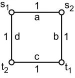
Nash equilibria may not exist It is not always the case that selfish agents can agree to pay for a network. There are instances of the connection game which have no pure Nash equilibria (equilibria in which players do not randomize over strategies). In Figure 1, there are 2 players, one wishing to connect node s1to node t1, and the other s2to t2. Now suppose that there exists a Nash equilibrium p. By Property 1 above, in a Nash equilibrium Gpmust be a forest, so assume without loss of generality it
s1 s2
t2 t1
1 1
1
1 a
c
d b
Figure 1: A game with no Nash equilibria.
s1
s2
t2
t1
6 5
5 3
3
s1
s2
t2
t1
5 3
3
a b
d e c
(a) (b)
1
Figure 2: A game with only fractional Nash equilibria.
strategy of only buying edge d and nothing else, which would connect his terminals with the player’s total payments being only 1. Therefore, no Nash equilibria exist in this example.
Fractional Nash equilibria When looking at the connection game, we might be tempted to assume that giving players the opportunity to share costs of edges is an unnecessary complication. However, sometimes players must share costs of edges for all players to agree on a network. There are game instances where the only Nash equilibria in existence require that players split the cost of an edge. We will call such Nash equilibria fractional and we will call Nash equilibria that do not involve players sharing costs of edges non-fractional.
InFigure 2(a) we have an example of a connection game instance where the only Nash equilibria are fractional ones. Once again, player 1 would like to connect s1 and t1, and player 2 would like to connect s2and t2. First, note that there is a fractional Nash equilibrium, as shown inFigure 2(b), with the contribution of player 1 (2) indicated with a thick black (gray) line. Here player 2 contributes 5 to edge e and player 1 contributes 1 to e and 3 to both of a and c. It is easy to confirm that neither player has an incentive to deviate.
N
1
s
1,...,s
Nt
1,...,t
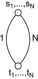
NFigure 3: A game with price of anarchy of N.
edge e. Given that edge e must be bought, it is clear that player 2 will only contribute to edge e. For a Nash equilibrium p to be non-fractional, this would mean that player 2 either buys edge e fully or buys nothing at all. Suppose player 2 buys e. The only response for which player 1 would not want to deviate would be to buy a and c. But then player 2 has an incentive to switch to either edge b or d. Now suppose player 2 does not buy e. Then the only response for which player 1 would not want to deviate would be to either buy a and b or buy c and d. Either way, player 2 does not succeed in joining his source to his sink, and thus has an incentive to buy an edge. Hence, there are no non-fractional Nash equilibria in this graph.
The price of anarchy We have now shown that Nash equilibria do not have to exist. However, when they exist, how bad can these Nash equilibria be? As mentioned above, the price of anarchy refers to the ratio of the costs of the worst (most expensive) Nash equilibrium and the optimal centralized solution. In the connection game, the price of anarchy is at most N, the number of players. This is simply because if the worst Nash equilibrium p costs more than N times OPT, the cost of the optimal solution, then there must be a player whose payments in p are strictly more than OPT, so he could deviate by purchasing the entire optimal solution by himself, and connect his terminals with smaller payments than before. More importantly, there are cases when the price of anarchy actually equals N, so the above bound is tight. This is demonstrated with the example inFigure 3. Suppose there are N players, and G consists of nodes s and t which are joined by 2 disjoint paths, one of length 1 and and one of length N. Each player has a terminal at s and t. Then, the worst Nash equilibrium has each player contributing 1 to the long path, and has a cost of N. The optimal solution here has a cost of only 1, so the price of anarchy is N. Therefore, the price of anarchy could be very high in the connection game. However, notice that in this example the best Nash equilibrium (which is each player buying 1/N of the short path) has the same
s
12
t
2t
t
3 32
3 2
3
2 2 2
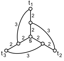
Figure 4: A single source game in which best response dynamics do not converge.
All the results in this section also hold if G is directed or if each player i has a maximum cost max(i) beyond which he would rather pay nothing and not connect his terminals.
3
Single source games
As we show inSection 5, determining whether or not Nash equilibria exist in a general instance of the connection game is NP-hard. Furthermore, even when equilibria exist, they may be significantly more expensive than the centrally optimal network. In this section we define a class of games in which there is always a Nash equilibrium, and the price of stability is 1. Furthermore, we show how we can use an approximation to the centrally optimal network to construct a(1+ε)-approximate Nash equilibrium in
poly-time, for anyε>0.
Definition 3.1. A single source game is a game in which all players share a common terminal s, and in addition, each player i has exactly one other terminal ti.
Before presenting our main result for this section, it is worth noting that even with single source games, best response dynamics (the process in which players alternate making improving moves when possible) does not necessarily converge to a pure Nash equilibrium at all. Three players all wish to connect to s. Consider an initial configuration in which each player pays fully for the cost 4 direct path from their terminal to s (although any non-fractional configuration will lead to the same conclusion). If player 1 is allowed to move, he will take the shortcut to the middle of player 3’s path, paying 3 to do so. Likewise, player 3 has an incentive to take a shortcut to the middle of player 2’s path. But doing so leaves player 1 disconnected, and thus player 1 will revert to his direct connection. Since the resulting configuration is simply a rotation of a previous configuration, it is not hard to see that this process will never terminate.
mechanisms [17]. The Marginal Cost (or VCG) mechanisms are very far from being budget balanced, i. e. the agents do not pay for even a constant fraction of the tree built. The Shapley value mechanism is budget balanced: the cost of each edge is evenly shared by the terminals that use the edge for their connection (i. e., the terminals in the subtree below the edge e). However, this method does not lead to a Nash equilibrium in our game: some players can have cheaper alternative paths, and hence benefit by deviating. Jain and Vazirani [24] give a truthful budget balanced cost-sharing mechanism to pay for the minimum spanning tree, which is a 2-approximate budget balanced mechanism for the Steiner tree problem. However, it is only a 2-approximation, and the cost-shares are not associated with edges that the agents use. Here we will show that while the traditional Steiner tree cost-sharing methods do not lead to a Nash equilibrium, such a solution can be obtained.
Theorem 3.2. In any single source game, there is a Nash equilibrium which purchases T∗, a minimum cost Steiner tree on all players’ terminal nodes.
Proof. Given T∗, we present an algorithm to construct payment strategies p. We will view T∗as being rooted at s. Let Te be the subtree of T∗ disconnected from s when e is removed. We will determine
payments to edges by considering edges in reverse breadth first search order. We determine payments to the subtree Te before we consider edge e. In selecting the payment of agent i to edge e we consider c0,
the cost that player i faces if he deviates in the final solution: edges f in the subtree Teare considered to
cost pi(f), edges f not in T∗cost c(f), while all other edges cost 0. We never allow i to contribute so
much to e that his total payments exceed his cost of connecting tito s.
Algorithm 3.3. Initialize pi(e) =0 for all players i and edges e.
Loop through all edges e in T∗ in reverse BFS order. Loop through all players i with ti∈Te until e paid for.
If e is a cut in G set pi(e) =c(e).
Otherwise
Define c0(f) =pi(f) for all f∈T∗ and
c0(f) =c(f) for all f ∈/T∗.
Define χi to be the cost of the cheapest path from s to
ti in G\ {e} under modified costs c0.
Define pi(T∗) =∑f∈T∗pi(f). Define p(e) =∑jpj(e).
Set pi(e) =min{χi−pi(T∗),c(e)−p(e)}.
end end end
We first claim that if this algorithm terminates, the resulting payment forms a Nash equilibrium. Consider the algorithm at some stage where we are determining i’s payment to e. The cost function
c0 is defined to reflect the costs player i faces if he deviates in the final solution. We never allow i to contribute so much to e that his total payments exceed his cost of connecting tito s. Therefore it is never
in player i’s interest to deviate. Since this is true for all players, p is a Nash equilibrium.
Te
Ai
ti e
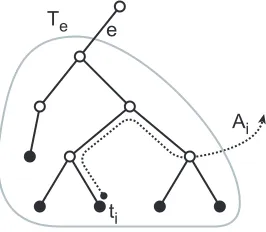
Figure 5: Alternative paths in single source games.
are unwilling to buy an edge e. Then each player has some path which explains why it can’t contribute more to e. We can use a carefully selected subset of these paths to modify T∗, forming a cheaper tree that spans all terminals and doesn’t contain e. This would clearly contradict our assumption that T∗had minimum cost.
Define player i’s alternative path Ai to be the path of cost χi found inAlgorithm 3.3, as shown in
Figure 5. If there is more than one such path, choose Aito be the path which includes as many ancestors
of tiin Teas possible before including edges outside of T∗. To show that all edges in T∗are paid for, we
need the following technical lemma concerning the structure of alternative paths.
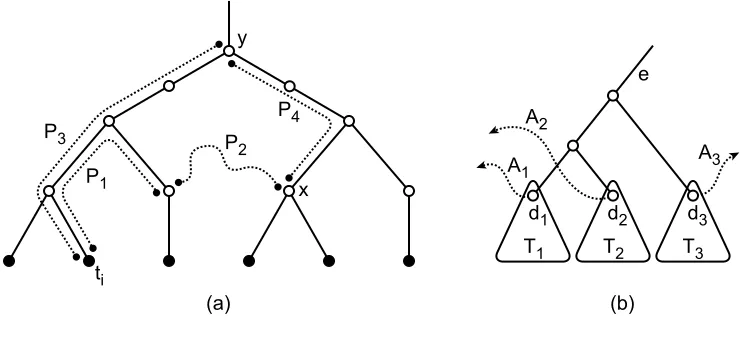
Lemma 3.4. Suppose Aiis i’s alternative path at some stage of the algorithm. Then there are two nodes
v and w on Ai, such that all edges on Ai from tito v are in Te, all edges between v and w are in E\T∗,
and all edges between w and s are in T∗\Te.
Proof. Once Aireaches a node w in T∗\Te, all subsequent nodes of Ai will be in T∗\Te, as all edges f
in T∗\Te have cost c0(f) =0 and the source s is in T∗\Te. Thus, suppose Aibegins with a path P1 in
Te, followed by a path P2containing only edges not in T∗, before reaching a node x in Te, as shown in
Figure 6(a). Let y be the lowest common ancestor of x and tiin Te. Define P3to be the path from tito y
in Te, and define P4to be the path from y to x in Te. We will show that by replacing P1∪P2with P3∪P4, player i would obtain a better deviation than Ai.
First, we prove that P1is strictly below y. If this were not the case, then P3is a subpath of P1, and so c0(P3)≤c0(P1). The modified cost of P4is always 0, as none of the edges in P4are on player i’s path from ti to s in T∗. Since P2 is disjoint from T∗, its modified cost is just the actual cost of the path P2, i. e., c0(P2) =c(P2). This cost is strictly positive (if there were any 0-cost edge in the graph, we could have simply contracted them before beginning our payment process). Therefore, the cost to agent i to purchase P1∪P2is strictly greater than the cost to purchase P3∪P4, and so Aicannot be a best deviation
path for agent i. Because of this contradiction, we may now assume that P1is strictly below y.
We now show that under the modified cost function c0, P3∪P4is at least as cheap as P1∪P2. Since
ti P1
P2 P4 P3
x y
T1 T2 T3
d1 d2 d3
A1 A2
A3 e
(b) (a)
Figure 6: Alternative path structure in the proof ofTheorem 3.2.
Consider the iterations of the algorithm during which player i could have contributed to edges in
P3. At each of these steps the algorithm computes a cheapest path from ti to s. At any time, player i’s
payments are upper bounded by the modified cost of his alternate path, which is in turn upper bounded by the modified cost of any path from tito s. In particular, player i’s payments on P3are upper bounded by the modified cost of the path P1∪P2, followed by a path in T∗ from x to s. The latter path from x to s has modified cost of 0, since we have not asked player i to contribute to any edges above y at this point. Therefore, i’s contribution to P3is always at most the modified cost of P1∪P2. This implies that
c0(P3∪P4) =c0(P3)≤c0(P1∪P2), as desired.
Thus, players’ alternative paths may initially use some edges in Te, but subsequently will exclusively
use edges outside of Te. We use this fact in the following lemma.
Lemma 3.5. Algorithm 3.3fully pays for every edge in T∗.
Proof. Suppose that for some edge e, after all players have contributed to e, p(e)<c(e). That is, the total payments currently being made by players in Te do not cover the cost of connecting these players
to T∗\Te. We will demonstrate how to rewire Te so as to connect all players in Te to T∗\Te without
increasing their payments, thus contradicting the minimality of T∗.
For each player i, call the highest ancestor of tiin Ai that is also in Tei’s deviation point, denoted di.
Let D be the set containing the highest deviation points in Te.
We modify T∗by replacing Te as follows: those players i whose alternative paths Ai are associated
with nodes in D deviate to Ai, as shown inFigure 6(b). All other players leave their payments unchanged.
Note that no player has increased his expenditures. If we can show that all terminals in Teare connected
Define Ti to be the subtree rooted at di. Consider any edge f in Ti. ByLemma 3.4, player i is the
only deviating player who could have been contributing to f . If i did contribute to f , then f must be on the unique path from tito diin Te, and hence f is in Ai. Thus Tiis fully paid for.
ByLemma 3.4, we know that Ai consists of edges in Ti followed by edges in E\T∗ followed by
edges in T∗\Te. The modified cost c0of edges in E\T∗is their actual cost. Thus i pays fully for a path
connecting Tito T∗\Te. Thus all terminals in Teare connected to T∗\Te, as desired.
Since we have also shown that the algorithm always produces a Nash equilibrium, this concludes the proof of the theorem.
We will now argue thatAlgorithm 3.3works even if the graph is directed. It is still the case that if the algorithm does succeed in assigning payments to all edges, then we are done. Hence, to prove correctness, we will again need only show that failure to pay for an edge implies the existence of a cheaper tree, thus yielding a contradiction. The problem is thatLemma 3.4no longer holds; it is possible that in a directed network, some of the players attempting to purchase an edge e have an alternative path which repeatedly moves in and out of the subtree Te. Thus, the argument is more complex, and requires
a slightly different definition for D.
Lemma 3.6. Algorithm 3.3fully pays for every edge in T∗for directed graphs.
Proof. Suppose the algorithm fails to pay for some edge e. At this point, every player i with a terminal in Tehas an alternative path Ai, as defined earlier. Define D to be the set of vertices contained in both Teand
at least one alternative path. Note that D contains all terminals that appear in Te. We now create D0⊆D
by selecting the highest elements of D; we select the set of nodes from D that do not have ancestors with respect to Tein D. Every terminal in Tehas a unique ancestor in D0with respect to Te, and every node in
D0can be associated with at least one alternative path.
For any node v∈D0, let Av be the alternative path containing v. If more than one such path exists,
simply select one of them. Define A0vto be the portion of this path from v to the first node in T\Te. Note
that A0v does not re-enter the subtree rooted at v, since if it did, we could find a shorter alternative path by shortcutting the distance between where A0ventered and left that subtree.
We can now form T0as the union of edges from T\Te, all paths A0v, and every subtree of Te rooted
at a node in D0. T0might not be a tree, but breaking any cycles yields a tree which is only cheaper. It is clear that all terminals are connected to the root in T0, since every terminal in Teis connected to
some node in D0, which in turn is connected to T\Te. Now we just need to prove that the cost of our new
tree is less than the cost of the original. To do so, we will show that the total cost of the subtrees below nodes in D0, together with the cost of adding any additional edges needed by the paths A0v, is no greater than the total payments assigned by the algorithm to the players in Te thus far. Hence it will be helpful
if we continue to view the new tree as being paid for by the players. In particular, we will assume that all players maintain their original payments for all edges below nodes in D0, and the additional cost of building any path A0v is covered by the player for which Av was an alternative path. It now suffices to
show that no player increases their payment.
v
ti
Av u P1
P2
P3
P4 v’
Figure 7: Alternative path structure in the proof ofLemma 3.6.
not be contained within the subtree rooted at v. If it is, then we are done, since in this case, player i’s new cost is at most the cost of Av, which is exactly i’s current payment.
Thus suppose instead that player i’s terminal lies in a subtree rooted at a different node v06=v∈D0
(this case is shown inFigure 7). Define u to be the least common ancestor of v and v0 in Te. Observe
that u can not be either v or v0, as this would contradict the minimality of the set D0. Define P1to be the current payments made by player i from its terminal to u, and let P2 be the current payments made by player i from u to e (inclusive). Define P3 as the cost of Av\A0v and let P4 be the cost of A0v. Note that
all costs are with respect to c0as defined in the algorithm, and as such, depend on both player i’s current payments, and those of the other players. By the definition of alternative path,
P1+P2=P3+P4.
Furthermore, since we have already successfully paid for a connection to u, we know that P3≥P1,since otherwise, when we were paying for the edges between v and u, player i would have had an incentive to deviate by purchasing P3and then using the path from v to u in Te, which would have been free for i.
Hence P4≤P2.
Therefore we can bound player i’s contribution to edges below D0 by P1(since u lies above v0), and we can bound player i’s contribution to A0vby P2. Taken together, we have that player i’s new cost has not increased. Thus in T0, no player has increased his payment, all terminals in Teare connected to T\Te,
and these edges are fully paid for. Since those same terminals did not fully pay for Te∪ {e}originally,
T0must be cheaper than T , but this is a contradiction.
We have shown that the price of stability in a single source game is 1. However, the algorithm for finding an optimal Nash equilibrium requires us to have a minimum cost Steiner tree on hand. Since this is often computationally infeasible, we present the following result.
Theorem 3.7. Suppose we have a single source game and an α-approximate minimum cost Steiner
tree T . Then for anyε >0, there is a poly-time algorithm which returns a(1+ε)-approximate Nash
Proof. To find a(1+ε)-approximate Nash equilibrium, we start by definingγ=εc(T)/((1+ε)nα).
We now useAlgorithm 3.3to attempt to pay for all butγ of each edge in T . Since T is not optimal, it is
possible that even with theγreduction in price, there will be some edge e that the players are unwilling
to pay for. If this happens, the proof ofTheorem 3.2indicates how we can rearrange T to decrease its cost. If we modify T in this manner, it is easy to show that we have decreased its cost by at leastγ. At
this point we simply start over with the new tree and attempt to pay for that.
Each call toAlgorithm 3.3 can be made to run in polynomial time. Furthermore, since each call which fails to pay for the tree decreases the cost of the tree byγ, we can have at most(1+ε)αn/εcalls.
Therefore in time polynomial in n,α anε−1, we have formed a tree T0with c(T0)≤c(T)such that the
players are willing to buy T0if the edges in T0have their costs decreased byγ.
For each player i and for each edge e in T0, we now create a new payment p0i(e)by increasing pi(e)
in proportion to player i’s total payments over T0such that e is fully paid for. In particular,
p0i(e) =pi(e) +γ
pi(T0)
∑jpj(T0)
.
Notice that players will now be paying for edges which they might not even use. Under p0, T0is clearly paid for. To see that this is a(1+ε)-approximate Nash equilibrium, note that player i did not want to
deviate before his payments were increased. If we let m0be the number of edges in T0, then i’s payments were increased by
p0i(T0)−pi(T0) =γ
pi(T0)
c(T0)−m0γm
0= εc(T)pi(T0)m0
(1+ε)nα(c(T0)−m0γ)
≤ εc(T)pi(T
0)
α(1+ε)(1−ε)c(T0)
≤εpi(T0).
Thus any deviation yields at most anε factor improvement.
Extensions Both Theorem 3.2 and Theorem 3.7 can be proven for the case where our graph G is directed, and players wish to purchase paths from tito s, although unfortauntely, the best-known
approx-imation algorithms for the directed problem is quite weak. Once we have shown that our theorems apply in the directed case, we can extend our model and give each player i a maximum cost max(i) beyond which he would rather pay nothing and not connect his terminals. It suffices to make a new terminal ti0 for each player i, with a directed edge of cost 0 to tiand a directed edge of cost max(i)to s.
4
General connection games
In this section we deal with the general case of players that can have different numbers of terminals and do not necessarily share the same source terminal. As stated before, in this case the price of anarchy can be as large as N, the number of players. However, even the price of stability may be quite large in this general case.
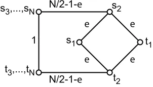
Consider the graph illustrated inFigure 8, where each player i owns terminals siand ti. The optimal
centralized solution has cost 1+3ε. If the path of length 1 were bought, each player i>2 will not want
to pay for anyεedges, and therefore the situation of players 1 and 2 reduces to the example inSection 2
s3,...,sN
t3,...,tN
s2
t2
s1 t1
N/2-1-e
1
e e e
e
N/2-1-e
Figure 8: A game with high price of stability.
path of length N−2. In fact, if each player i>2 buys 1/(N−2)of this path, then we have a Nash equilibrium. Therefore, for any N>2, there exists a game with the price of stability being nearly N−2. Because the price of stability can be as large as Θ(N), and sometimes pure Nash equilibria may not exist at all, we cannot hope to be able to provide cheap Nash equilibria for the multi-source case. Therefore, we consider how cheapα-approximate Nash equilibria with smallα can be, and obtain the
following result, which tells us that there always exists a 3-approximate Nash equilibrium as cheap as the optimal centralized solution.
Theorem 4.1. For any optimal centralized solution T∗, there exists a 3-approximate Nash equilibrium such that the purchased edges are exactly T∗.
We prove this theorem inSection 4.3using the sufficient conditions for an approximate Nash equi-librium ofTheorem 4.2. InSection 4.2we address the key special case where the underlying graph is a path, which is then extended to the general case via a simple induction. InSection 4.4we give lower bounds and a polynomial time algorithm for finding an approximate Nash equilibrium.
4.1 Connection sets and sufficient conditions for approximate Nash equilibria
Given a set of bought edges T , denote by a stable payment pifor player i a payment such that player i has
no better deviation than pi, assuming that the rest of T is bought by the other players. A Nash equilibrium
must consist of stable payments for all players. However, what if in some solution, a player’s payment
piis not stable, but is a union of a small number of stable payments? This implies that each player’s best
deviation is not much less than its current payment. Specifically, we have the following general theorem.
Theorem 4.2. Suppose we are given a payment scheme p= (p1, . . . ,pN), with the set of bought edges
T . Further, suppose that for all i, pi can be decomposed into α sub-payments p1, . . . ,pα (together
summing to pi) such that each of sub-payment is a stable payment for i with respect to T . Then p is an
α-approximate Nash equilibrium.
Proof. Let p0ibe the best deviation of player i given p, and let p1, . . . ,pαbe the stable payments which together sum to pi. The fact that p0i is a valid deviation for i means that the set of bought edges T with
only pays for pj and the rest of T is bought by other players, then the best deviation of i is at least as expensive as pj. In this case, p0iis still a possible deviation, since if taking out piand adding p0iconnects
the terminals of i, then so does taking out pj and adding p0i. Therefore, we know that the cost of p0iis no smaller than the cost of any pj, andα·cost(p0i)≥cost(pi), where cost(pi)denotes the total cost for i of
playing strategy pi.
Notice that the converse of this theorem is not true. Consider an example where player i is contribut-ing to an edge which it does not use to connect its terminals. If this edge is cheap, this would still form an approximate Nash equilibrium. However, this edge would not be contained in any stable payment of player i, so piwould not be a union of stable payments.
To proveTheorem 4.1, we will construct a payment scheme on the optimal centralized solution such that each player’s payment is a union of 3 stable payments. The stable payments we use for this purpose involve each edge being paid for by a single player, and have special structure. We call these payments
connection sets. Since there is no sharing of edge costs by multiple players in connection sets, we will
often use sets of edges and sets of payments interchangeably. T∗ below denotes an optimal centralized solution, which we know is a forest.
Definition 4.3. A connection set S of player i is a subset of edges of T∗such that for each connected component C of the graph T∗\S, we have that either
(1) any player that has terminals in C has all of its terminals in C, or
(2) player i has a terminal in C.
Intuitively, a connection set S is a set such that if we removed it from T∗and then somehow connected all the terminals of i, then all the terminals of all players are still connected in the resulting graph. We now have the following lemma, the proof of which follows directly from the definition of a connection set.
Lemma 4.4. A connection set S of player i is a stable payment of i with respect to T∗.
Proof. Suppose that player i only pays exactly for the edges of S, and the other players buy the edges in T∗\S. Let Q be a best deviation of i in this case. In other words, let Q be a cheapest set of edges such
that the set(T∗\S)∪Q connects all the terminals of i. To prove that S is a stable payment for i, we need
to show that cost(S)≤cost(Q).
Consider two arbitrary terminals of some player. If these terminals are in different components of
T∗\S, then by definition of connection set, each of these components must have a terminal of i.
There-fore, all terminals of all players are connected in(T∗\S)∪Q, since(T∗\S)∪Q connects all terminals of i. Since T∗is optimal, we know that cost(T∗)≤cost((T∗\S)∪Q). Since S⊆T∗and Q is disjoint from
T∗\S, then cost((T∗\S)∪Q) =cost(T∗)−cost(S) +cost(Q), and so cost(S)≤cost(Q).
As a first example of a connection set consider the edges Siof T∗that are used exclusively by player
i. More formally, let Tibe the unique smallest subtree of T∗containing all terminals of player i, and let
Q(u1)
u2
u1 u3 u4
vn Q(u2) Q(u3) Q(u4)
Q(u1)
u3
u2 u4 u5
Q(u2) Q(u3) Q(u4)
(c) (b)
u6 u5 Q(u1)
u2
u1 u3 u4
vn Q(u2) Q(u3)
Q(u4)
(a)
v1
u1 v1
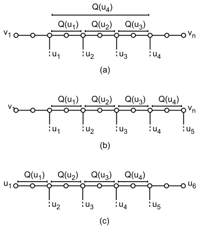
Figure 9: The paths Q(u)for a single player i. (a) i has no terminal in Un(b) i has a terminal in Un(c) i
is the special player ofLemma 4.11that has terminals both in v1and vn.
Proof. Suppose to the contrary that there are at least two components of T∗\Si that contain terminals t1 and t2 of some player j6=i. Since T∗ is a tree that connects all terminals, this means that the path in
T∗between t1and t2must also be contained in Tj. But this implies that the edges of Siwhose removal disconnected this path also belong to Tj, which contradicts the definition of Si.
Each player i will pay for this connection set, the set of edges used only by player i. We want each player to pay for at most 2 additional connection sets. Without loss of generality we can contract the edges now paid for, forming a new tree T∗ which the players must pay for. For the remainder of this section we will assume that each edge belongs to at least two different Ti’s, and will have players pay for at most two connection sets.
4.2 Approximate Nash equilibrium in paths
In this subsection we consider the key special case when the tree T∗is a path P. In the next section we use induction to extend the proof to the general case.
We will use vk, k=1, . . . ,n to denote the nodes on the path P in the order v1, . . . ,vn, and will refer
to the terminals in this order, for example, the “first” terminal of player i will mean the one closest to v1. Denote the set of all terminals located at vkby Uk, and assume that each edge is in at least two different
Ti’s as mentioned above.
1 1
2 2
3
34 4 5 5
6 6
Figure 10: The bold edges along the path form a single connection set connecting two neighboring terminals of players 1 and 2.
set of edges Q(u)as the possible edges that can be associated with u. For every terminal u∈Ukowned
by a player i, with k6=n, define a subpath Q(u)as follows (illustrated onFigure 9(a)). If i owns another terminal in U`with` >k, then set Q(u)to be the subpath of P from vkto the first such node v`. If there is no such node (because u is i’s last terminal in P), set Q(u)to be the subpath of P starting at the first terminal of i, and ending at vk. Notice that Q(u)is not defined for u∈Un, so if i has a terminal in Un,
the Q(u)paths for terminals of i will look likeFigure 9(b).
A key observation about the Q sets is that if a player i pays for one edge in each Q(u)(excluding the one belonging to the last terminal) the resulting set forms a connection set.
Lemma 4.6. Consider a payment Si by player i that contains at most one edge from each path Q(u), where u are terminals of i excluding the last terminal of i. Then, Si forms a connection set.
Proof. Every component of P\Si contains a terminal of i, since there is a terminal of i between every two Q(u)’s for u belonging to i, as well as before the first such Q(u), and after the last one. This means that Si is a single connection set.
Unfortunately, we cannot assign each edge to a different terminal, as shown by the example of
Figure 10. The bold edges in this example are used only by players 1 and 2, and belong to the Q paths of the first terminals of players 1 and 2. This leaves us with three edges and only two terminals to assign them to. However, note that the set of bold edges is a single connection set by itself, even though it contains more than one edge in every Q path. We say that a set L of edges along the path is coupled if all the edges e∈L belong to the exact same sets Q(u)for u∈ ∪Uk. We need to extend our ideas so far
to allow us to assign such coupled sets of edges to a terminal, rather than just assigning a single edge.
Definition 4.7. A max-coupled-set L is a maximal set of edges of P such that for every edge e∈L, the
set of paths Q(u)that contain e is exactly the same, for u∈S Uk.
The key property of max-coupled-sets is they form a connection set between two consecutive termi-nals of one player.
Lemma 4.8. Consider a max-coupled-set L, and order all components C of P\L along the path. For all components C except the two end components, any player that has terminals in C has all of its terminals in C.
to some path Q(u) with u a terminal of j, then this gives us a contradiction, since the paths Q(u)for terminals of j change at t, and never become the same. This contradicts the fact that L is a coupled set, since both edges of L must be in exactly the same Q paths. On the other hand, if the earlier edge of L adjacent to C does not belong to any path Q(u)with u a terminal of j, then for the edges of L on the other side of C to belong to the same Q paths, it must be that all terminals of j are inside C, as desired.
This implies the following extension ofLemma 4.6
Lemma 4.9. Consider a payment Si by player i that contains at most one max-coupled-set from each path Q(u), where u are terminals of i excluding the last terminal of i along the path. Then, Si forms a connection set.
Proof. We must prove that every component of P\Siobeys one of the two properties from the definition
of a connection set. Consider a component of P\Si that does not contain a terminal of i. By the argu-ment inLemma 4.6, this component must be bordered by edges of the same max-coupled-set, and by
Lemma 4.8, this component satisfies the first property in the definition of a connection set.
Now we are ready to prove our main result for paths. To help with the induction proof appearing in
Subsection 4.3for the case of trees, we need to prove a somewhat stronger statement for paths.
Theorem 4.10. Assume the optimal tree T∗ is a path P, and each edge of P is used by at least two players. There exists a payment scheme fully paying for path P such that each player i pays for at most 2 connection sets. Moreover, players with terminals in Unpay for at most 1 connection set.
Proof. In our payment, we will assign max-coupled-sets of edges to terminals u. ByLemma 4.9the edges Siassigned to the terminals of player i, excluding the last terminal of i, form a single connection set. For players that do not have a terminal in Un the max-coupled-set assigned to the last terminal
forms a second connection set. Since a max-coupled-set is a connection set by itself, this would meet the conditions of the Theorem.
To form this payment, we form a bipartite matching problem as follows. Let Y have a node for each max-coupled-set of edges in P, and let Z be the nodes of v1, . . . ,vn−1 of P. Form an edge between a node vk∈Z and node L∈Y if there exists some terminal u∈Uksuch that L⊆Q(u). This edge signifies
that some player owning u∈Uk could pay for L. In addition, if u∈Uk is the last terminal of a player
i, but k6=n, then we also form an edge between vk ∈Z and L∈Y if L⊆Ti. These edges signify the
“additional” max-coupled-set that this player might pay for since it owns no terminals in Un.
We claim that this graph has a matching that matches all nodes in Y , and we will use such a matching to assign the max-coupled-sets to terminals according to the edges in this matching. To prove that such a matching exists, we use Hall’s Matching Theorem. For X⊆Y , define∂(X)to be the set of nodes in Z
which X has edges to. According to Hall’s Matching Theorem, there exists a matching in this bipartite graph with all nodes of Y incident to an edge of the matching if for each set X⊆Y ,|∂(X)| ≥ |X|. To
prove that this condition is satisfied, arrange the edges E(X)in the max-coupled-sets X in the order they appear in P. We want to show that between every two max-coupled-sets of X , there is a node belonging to∂(X). This will yield|X| −1 nodes in∂(X). Then we show that there is an additional node in∂(X)
Consider some edge e of E(X)that belongs to a max-coupled-set L, and suppose a previous edge e0 in E(X)belongs to a different a max-coupled-set L0. Since these are different and maximal coupled sets, there must be some path Q(u)that contains exactly one of e,e0. The player corresponding to this path
Q(u)must have a terminal between e and e0that is in the set∂(X).
We need to prove that there is an additional node in∂(X) before the set E(X). Let L be the first
max-coupled-set of X that appears in P. The player corresponding to a path Q(u) containing L must have a terminal in∂(X)before L.
Therefore, |X| ≤ |∂(X)|for all X ⊂Y , and hence there always exists a matching that covers the
max-connection-sets Y .
This finishes our proof that if T∗is a path, then there exists a 3-approximate Nash equilibrium that purchases exactly T∗(2-approximate when all edges in T∗ are used by at least two players). To prove the general case, however, we need the following strengthening.
Lemma 4.11. Suppose there exists a player i with a terminal s∈U1and a terminal in Un. Then there
exists a payment scheme as inTheorem 4.10and moreover i has at least 2 terminals in the component of P\Sicontaining vn.
Proof. We change the definition of Q(u)for the terminals of i, as shown inFigure 9(c). We let Q(u)be the path immediately to the left of u, until it reaches the next terminal of i.
We show that the proof ofTheorem 4.10goes through in this case with minor changes. First note that the max-coupled-sets are exactly the same sets as before. Note that the max-coupled-sets assigned to player i now will form a single connection set, and further the last terminal of i before Unwould be in
the component of P\Sicontaining vn, as we desired.
We must now verify that the bipartite graph formed in the proof of Theorem 4.10 actually has a matching that covers all of the max-coupled sets. To do this, we need to prove that|X| ≤ |∂(X)|for a
set X⊂Y , which we do once again by showing that between every pair of max-coupled-sets in X there
exists a node of∂(X), and there is a further node of∂(X)in front of the set E(X).
As before, if we have two edges e and e0 that belong to two different max-coupled-sets, then any player j that has a set Q(u)containing exactly one of e and e0 must have a terminal in∂(X) between
e and e0. To see that we have a node in∂(X)before E(X)let L be the first max-coupled-set of X that appears in P, the let j be the player corresponding to a path Q(u) containing L. If j6=i then j has a
terminal in∂(X)before L. Recall that each edge is used by at least two players so we can select a Q(u)
set containing L that belongs to a player j6=i.
We can now continue with the process given in the proof of Theorem 4.10 to form the desired payment scheme.
We will need the following further observation about the proof: in the proof at most one terminal is assigned any set of edges among the terminals in each set Uk, for any node vk of the path.
Lemma 4.12. There exists a set
A={u1,u2, . . . ,un−1}
with uk∈Uk such that only the terminals u1, . . . ,un−1 are assigned max-coupled-sets in the payment
4.3 Proof ofTheorem 4.1(Existence of 3-approx Nash equilibrium)
In this subsection, we prove that for any optimal centralized solution T∗, there exists a 3-approximate Nash equilibrium such that the purchased edges are exactly T∗. For simplicity of the proof, we assume that T∗is a tree, since otherwise we can apply this proof to each component of T∗.
Recall that we used Ti to denote the unique smallest subtree of T∗ which connects all terminals of player i. We formed the first connection set usingLemma 4.5by the edges that belong to a single Ti. Contracting these edges, we can assume that all edges are used by at least two players, and we will construct a payment scheme in which each player is paying for at most 2 connection sets.
Intuition and proof outline The idea of the proof is to select two terminals of a player i, let P be the path connecting them in T∗, and let t1=v1, . . . ,vn=tndenote the nodes along the path P. We apply the
special case for paths,Lemma 4.11, to the path P with all players j with sets Tj∩P nonempty. Then we
apply the induction hypothesis for each subtree rooted at the nodes vk of path P, where we use the one
player j (byLemma 4.12) that has a max-coupled-set assigned to node vk as a “special” player, whose
two terminals we select to form a path as above.
To make the induction go through we need a stronger version of Theorem 4.1 analogous to the stronger version of the path lemma (Lemma 4.11).
Theorem 4.13. Assume each edge of the optimal tree T∗ is used by at least two players, let t be a terminal, and i a player with terminal t. Then there exists a way to pay for T∗by assigning at most two connection sets to each player, so that the following hold:
(1) each player j that has t as a terminal has at most one connection set assigned,
(2) for the connection set Si assigned to player i the set T∗\Si has an additional terminal of i in the component containing terminal t.
Proof. Let s be another terminal of player i, and let P be the path connecting s and t in T∗. Let s=
v1, . . . ,vn=t be the sequence of nodes along P, and let Tk∗be the subtree of T∗\P rooted at node vk.
Now we define a problem on path P, and subproblems for each of the subtrees Tk∗. First we define the problem for path P. A player j will have a terminal at node vkif player j has a terminal in the subtree
Tk∗. With this definition, each edge of P is used by at least two players. We applyLemma 4.11with i as the special player (by choice of the path i has both vnand v1as terminals in the induced problem on the path). We assign each player connection sets.
Next we will define the problems on the trees Tk∗. For this subproblem we say that vkis a terminal
for any player that has a terminal outside of the subtree Tk∗. We use the induction hypothesis to assign connection sets to players in Tk∗. Recall that byLemma 4.12at most one player, say player ik, is assigned
a max-coupled-set to a terminal in vk on the path problem. We use vk as the terminal t in the recursive
call, and ikas the special player.
To finish the proof we need to argue that the assignment satisfies the desired properties of our theo-rem. We will need to have a few cases to consider.
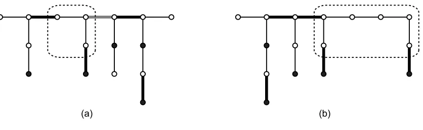
(a) (b)
Figure 11: Sets assigned to a player that do not form one connection set. The nodes in dark are terminals for one player j, and dark edges are assigned to this player with the grey edge assigned to the last terminal of j along the path. (a): the case when t6∈Tj, and a set (the grey edge) is assigned to the last terminal of j along P. (b): the case when no connection set is assigned to the last terminal of j along P.
Now consider a player j that has t as a terminal, but j6=i. For each subtree that has terminals of
player j the recursive call has assigned at most one connection set to player j, and we may have also assigned a connection set at path P. Note that in the path P the player j owns terminal t, so its last terminal is t, and has no set Q(t). We claim that combining all the sets j is paying for into one set Sj forms a single connection set. To see why consider the connected components of Tj\Sj. Connected components contained in a subtree Tk∗ satisfy one of the connection set properties by the induction hypothesis. If a terminal u at a node vk of the path problem was assigned a max-coupled-set along the
path P then in the recursive call we guaranteed that player j has a terminal connected to the root vk, so
the component containing vkhas a terminal in Tj\Sj. Finally, the last component along the path contains
the terminal t.
A similar argument applies for the special player i: the union of all connection sets assigned to i for the path and for the recursive calls combines to a single connection set Si that satisfies the extra requirement that set T∗\Sihas an additional terminal in the component containing terminal t.
Finally, consider a player j where t is not a terminal of j (though it may be included in Tj). As before
for each subtree that has terminals of player j the recursive call has assigned at most one connection set to player j, and we may have also assigned a connection set at path P. This case differs from the previous ones in two points. First, if t6∈Tj then the last node v
kj of T
j along the path may have an
extra connection set assigned to it; second, the node t is not a terminal for player j. As a result of these differences, combining all the sets assigned to player j to a single set Sj may not form a single connection set. Consider the connected components of Tj\Sj. Connected components fully contained in a subtree Tk∗satisfy one of the connection set properties by the induction hypothesis. Most components that intersect the path P must also have a terminal of player j: if a terminal u in the path problem at a node vk was assigned a connection set along the path P then in the recursive call we guaranteed that
player j has a terminal connected to the root vk, hence the component containing node vk has a terminal
. . . . . .
s1 s2 s3 sN t1 t2 t3 tN
Figure 12: A graph where players must pay for at least 3 connection sets.
However, there can be components of Tj\Sj intersecting the path P that do not satisfy either of the connection set properties. If vkj is the last node along the path P in T
j, then if v
kj has a max-coupled-set assigned to player j (e. g., if vkj 6=t) then the component(s) of T
j\Sj adjacent to this max-coupled-set
may not satisfy either of the connection set properties. Otherwise, the last component along the path
P may not satisfy these properties. SeeFigure 11 for examples for each possibility. In Figure 11(a), the grey edge is the max-coupled-set assigned to vkj, which results in the highlighted component not having any terminals of j. InFigure 11(b), nothing is assigned to vkj, and this also results in the high-lighted component not having any terminals of j. Notice, however, that all other components obey the connection set properties since they each have a terminal of j. In either case (whether vkj has a max-coupled-set assigned to it or not), removing one of the max-max-coupled-sets Lj(the one assigned to vkj, or one bordering the final component along P with no terminals) results in a connection set ¯Sj=Sj\Lj,
and the max-coupled-set Lj alone forms a second connection set.
4.4 Extensions and lower bounds
We have now shown that in any game, we can find a 3-approximate Nash equilibrium purchasing the optimal network. We proved this by constructing a payment scheme so that each player pays for at most 3 connection sets. This is in fact a tight bound. In the example shown inFigure 12, there must be players that pay for at least 3 connection sets. There are N players, with only two terminals (si and ti) for each
player i. Each player must pay for edges not used by anyone else, which is a single connection set. There are 2N−3 other edges, and if a player i pays for any 2 of them, they are 2 separate connection sets, since the component between these 2 edges would be uncoupled and would not contain any terminals of i. Therefore, there must be at least one player that is paying for 3 connection sets.
This example does not address the question of whether we can lower the approximation factor of our Nash equilibrium to something other than 3 by using a method other than connection sets. As a lower bound, inSection 5we give a simple sequence of games such that in the limit, any Nash equilibrium purchasing the optimal network must be at least(3/2)-approximate.