An accurate algorithm of numerical integration for computing seismic responses of inelastic structures

(1)

DOI: https://doi.org/10.30880/ijie.2018.10.02.016

An accurate algorithm of numerical integration for computing

seismic responses of inelastic structures

Masato Miyahara

1

_{, Katsushi Ijima}

1

_{, Hiroyuki Obiya}

1

_{, Muhammad Nizam bin}

Zakaria

2

1_{Department of Civil Engineering and Architecture, Graduate School of Science and Engineering, Saga University, 1,}

Honjo, Saga, 840-8502, Japan

2_{Department of Structural and Material Engineering, Faculty of Civil & Environmental Engineering, University Tun}

Hussein Onn Malaysia, 86400 Parit Raja Batu Pahat, Johor Darul Ta’zim, Malaysia Received 01 January 2018; accepted 15 April 2018, available online 07 May 2018

1. Introduction

The seismic proofs in Japan of bridges and buildings subjected by a strong earthquake are permitted to be over the yielding but must not be brought to the ultimate. The proofs need to evaluate the inelastic seismic responses of the structures [1], [2]. Therefore, many experimental researches on RC structures and steel structures were conducted for developing exact inelastic models of them. It has been, however, occasionally heard that the dynamic responses experimentally measured of real structures over the yielding disagreed with the computational results. This indicates that the algorithm of a numerical integration, that has not so far paid attention to, may be inappropriate in the computation.

Many methods of numerical integrations have been proposed for solving equations of motions. If we address methods for computing the inelastic seismic response of structures, the method of Newmark β=1/4 is the most popular method [4]. The method has no condition for computational stability, so that the method can directly and stably solve the equations of the motions. Further, when the method is applied to a linear problem filtering high frequency response, the result computed by enough short using time interval is almost equal to the result by the method of Newmark β=1/6. Since the method of β=1/6 applied to linear problems surely gives exacter responses than that by the method of β=1/4, this may be giving the method of β=1/4 assurance. However, there is a possibility that the response considerably includes

accumulative errors produced from high frequency components that do not diverge in the method of β=1/4 but surly possess errors, because of solving directly the equation of the motion unrestricted by frequency area.

The paper develops an algorithm for filtering high frequency components. The algorithm enables the method of numerical integration that is accurate but restricted within very small time interval for stably computing the inelastic seismic responses. The paper applies the method of modal analysis to the algorithm. The method of Newmark β=1/6 stably gives the inelastic seismic response without leading to divergence. The comparison between several seismic responses indicates that directly solving the equation of the motions will be inappropriate.

2. Modal Analysis for Computing Inelastic

Seismic Response

The equation of the motion expressing the seismic response at the time tm of an inelastic structure in three-dimensional space is,

, (1) where M: the mass matrix of the structure, C: the damping matrix possible to be arbitrarily composed, though the paper uses the Rayleigh damping C



M



Km , where ν and μ are constants. Moreover, Se,m: the end force vector of the element e,

Abstract: The paper proposes an algorithm that makes numerical integrations with conditions for stability to be usable for computing inelastic seismic responses of structures. The numerical integrations with conditions cannot be applied to solving directly the equation of the motion. These numerical integrations, however, give exacter results in linear seismic responses than that by the numerical integrations without any conditions. The method of modal analysis can clear the condition by applying the eigenvalue analysis to the equation of the motion expressed by the tangent stiffness in the inelasticity. The paper shows considerable difference between the result by the numerical integration with conditions and that without any condition, and the former result will be exacter than the latter from several proofs in the discussion.

(2)

e: the transforming matrix that changes the end forces to the forces in the universal coordinate, : the input acceleration at all the nodes, : the three components of the ground acceleration, : the nodal acceleration vector, : the nodal velocity vector.

Differentiating the third term in equation (1) gives the tangent stiffness Km at the timetm, that is,

m m e m , e

e

S

K



u



_













_

_

, (2) where



um is the infinitesimal increment of the nodal displacement.

If we assume that the equation of the motion during the time interval Δt from tm to tm1 is linear by using the

tangent stiffness Km, the method of modal analysis can be applied to the equation of the motion. The eigenvalue analysis of the free vibration expressed by M and Km yields the diagonal matrix m consisting of the square of the natural circular frequencies and the modal matrix Xm composed by the displacement modes dominating the responses of the structure.

The increment of the nodal displacement u in Δt is expressed from the modal analysis, as follows:

uXm Xm(m1 m), (3) where  is the increment of the normal coordinate vector in Δt.

The increment of the nodal velocity and that of the nodal acceleration are similarly obtained by differentiating equation (3).

Changing the increments of the nodal response into the increments of the normal coordinates yields the differential equation of the normal coordinates, as follows:

, (4) where I is the unit matrix and m is the matrix composed by the participation factors.

When the method of Newmark β is applied to equation (4), the increments of the normal coordinates is,

(0)

2 _2β 1 Δ

μ 2Δ ν Δ 1 β 1 _                _         _ m t t t I

. (5) Since the structure is inelastic, the increment (0) in equation (5) obtained from the linear analysis does not generally fulfill the equation of the motion at the time

1 

m

t . Therefore, adding corrections to the prediction (0)_{yields more accurate response. The correction is}

derived from the following. The prediction determines the

nodal displacement at the time t_m_₁ , and the displacement changes the tangent stiffness to K_m(1)1. The

eigenvalue analysis of M and K_m(1)_₁ gives the new diagonal matrix m(1)1 and the new modal matrix X(1)m1.

When the modal matrix changes, the normal coordinates change from (0) to (1) by applying the normalization.

The correction



(1) added to the increment of the normal coordinates (1)_{is obtained as the solution of}

the following linear equation,

(1) 1 (1)T 1 (1) (1) 1

2 _2β 1 δ δ

μ 2Δ ν Δ 1 β 1                  _         _ m m m t t

t I  X U ,

(6) where



U(1)_m_₁ expressing the unbalanced force vector at the time t_m_₁ is,

(7) If the equivalent force X_m(1)T1



U(1)m1 becomes less

than the allowable value, we can estimate the solution to be convergent.

3. Computational Example and Discussion

3.1 Computational model

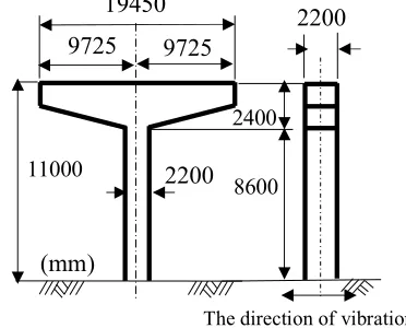
The proposed method is applied to the frame structure of the steel pier shown in Fig. 1. The pier fixed at the base plate is 11m in height and 126kN of the weight of the upper part on the ground. The top of the pier supports the girder of 957kN in weight. The computational model is the steel pier divided into 19 elements in the computation. Each element is the bar model that the bending deformation is only inelastic and the others are elastic. The elongation stiffness of the column part is 64312.5MN, and the shearing stiffness is 12290MN.

The bending stiffness before/after the yielding are 49021.56 MNm and 5071.8 2 MNm respectively, and 2

Fig. 1Steel pier used in the computation.

2200

19450

9725

11000

The direction of vibration 8600

2400

(3)

the bending moment at the yielding is 5MNm. The hysteresis loop of the bending behavior of inelasticity is defined as shown in Fig. 2 that expresses the relation between the bending moment and the curvature. Fig. 2 itself is the hysteresis loop in the bending behavior of the element on the base obtained from computing the response of the steel pier subjected by the earthquake.

The paper uses a uniform curvature element that would be the simplest model in various inelastic models already proposed. Even if the inelastic model is simple but appropriate, the frame model composed of plenty of fine elements will simulate nearly real phenomena. Further, since the purpose of the paper is to estimate algorithms of numerical integrations, it is allowable to select the simplest inelastic model.

The damping constant existing during the oscillation of the steel pier except the damping resulted from the inelasticity is defined as the Rayleigh damping in the computation, and the constants are ν0.114 1/sec. and

0.001157

μ sec.. These constants give the pier the damping effect nearly equal to the damping constant 0.02 in the frequency area from 0.5Hz to 10Hz.

3.2 Input acceleration of earthquake

The input acceleration used in computing the inelastic seismic response of the pier is shown in Fig. 3 that is NS component in the acceleration records of Hyogo-ken Nanbu Earthquake (1995) measured at Kobe station of Japan Meteorological Agency. The acceleration record is commonly being used for seismic proofs of bridges and buildings in Japan [1], [2]. The study also used some other strong-motion records obtained from National Research Institute for Earth Science and Disaster Resilience, NRIESDR’s home page [5] and computed the responses of the pier. Since those computational results were qualitatively similar to the following results, the paper is missing them.

3.3 Algorithms of numerical integration

compared

The paper compares the three algorithms that are the modal analysis with β=1/6, the modal analysis with β=1/4 and the direct solution with β=1/4 that is the method solving directly equation (1). All the conditions except the algorithms of numerical integration are the same in the computations.

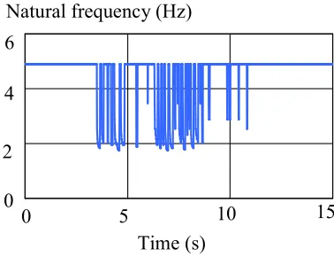
The natural frequencies in the lateral motion of the pier in the elastic state are the first of 4.899Hz, the second of 37.24Hz and the third of 124.3Hz. Fig. 4 shows the change of the first natural frequency during the oscillation of the pier. Naturally, the deterioration of the bending stiffness decreases the natural frequencies. The first natural frequency decreases from 4.899Hz to around 1.9Hz. Since main frequency area of earthquakes is generally less than 10Hz, the modal analysis uses only the first mode enough. Even if the pier was over the yielding, the natural frequency of the second mode was over 10Hz. Therefore, the method of the modal analysis did not need the modes over the first mode in this example.

The direct solution with β=1/4 does not use an algorithm of prediction/correction, but use the secant stiffness obtained from the two states of the bending at the times of t_m and tm₁. The direct solution iteratively

changes the secant stiffness from the state of the time

Curvature (10

-4

_/m)

Bending moment

(MNm)

5

10 -10

-5

-12

₁₂

Fig. 2The hysteresis loop in the bending behavior of the element on the base.

6

0 -6

0

Fig. 3 NS component in the acceleration records of Hyogo-ken Nanbu Earthquake (1995).

Acceleration (gal)

Time (s)

10

15

5

0 -500

-1000

500 1000

0

2

10

15

4

6

0 Natural frequency (Hz)

0 Time (s)

Fig. 4 Fluctuation of the first natural frequency of the pier during the inelastic response.

(4)

1 

m

t renewed, and the unbalanced forces of equation (7) more steadily converge in the iteration than using any algorithm of prediction/correction. The allowable unbalanced force in the direct solution is 0.01N.

3.4 Computational results

Fig. 5 shows the time-history responses of the displacement at the top of the pier computed by the three methods. The time interval is Δt=0.001 seconds, and the response by the modal analysis of β=1/4 almost agrees with that by the modal analysis of β=1/6, while does not agree with the response by the direct solution by β=1/4. The phases in the response wave by the direct solution seem to agree with that by the modal analysis, but the maximum peak by the direct solution is not only larger than those by the modal analysis but the latter part in the response is also.

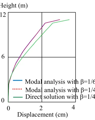
Fig. 6 shows the maximum of the lateral displacement at each node during the oscillation. The computation uses the time interval Δt=0.001 seconds,

because the time interval or less gives exact results, as shown by the following figures. The deformation by the displacement is similar to the first mode of the displacement. Comparison of the displacements by the

three methods reveals that the response by the direct solution is largest and that the two methods of modal analysis agree with each other.

Fig. 7 shows variations of the maximums of the displacement at the top of the pier according to the time interval. When the time interval becomes smaller and smaller, the maximums by the two methods of modal analysis are gradually close and converge on nearly the identical value. However, the maximum by the direct solution in Fig. 7 changes also, but the fluctuation is small. This convergent process to the time interval indicates that the maximums by the modal analysis will be exacter than that by the direct solution. Because, when we apply the two methods of Newmark β=1/4 and β=1/6 to the sinusoidal responses of a system of one degree of Fig. 5The time-history responses of the displacement at the top in the pier.

4

0

5

10

15 Displacement (cm)

2 -2

-4

Time (s)

Modal analysis with β=1/4

Modal analysis with β=1/6

Direct solution with β=1/4

0

Fig. 6 The maximums of the displacement of each node.

0

2

4

6

0 Height (m)

Displacement (cm)

Modal analysis with β=1/4

Modal analysis with β=1/6

Direct solution with β=1/4

12 Displacement (cm)

0.005 0.0005

Modal analysis with β=1/4

Modal analysis with β=1/6

Direct solution with β=1/4

Time interval Δ

t

(s)

8

4

0

0.01

(5)

freedom, both responses with sufficiently small interval of time agree well with the analytical solution that is exact. Since the modal analysis uses only the first mode in the computation in consideration of the frequency area

of the earthquake, the computation removes modes with high frequency.

On the other hand, the response by the direct solution implicitly includes components of high frequency. The errors caused by the components of high frequency will not be so small, because the maximum by the direct solution is so different from that by the modal analysis.

Fig. 8 showing the maximum of the acceleration at the top of the pier indicates that the acceleration by the direct solution agrees well with that by the modal analyses. If using another seismic wave to the computation, however, we obtained different results from Fig. 8. Therefore, when the maximum of the response early appears in the time-history, the value of the maximum by the direct solution will be accurate.

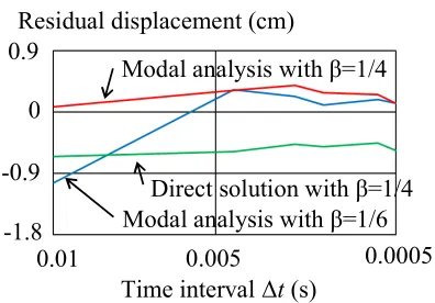
In the residual displacement at the top of the pier after the oscillation over shown in Fig. 9, the variations according to the time interval are large, but the results of the modal analysis agree with each other at Δt=0.001 seconds. On the other hand, the result of the direct solution does not seem to be convergent. This may be why the errors caused by high frequency gradually accumulate together with the procession of time.

4. Conclusion

Although the accuracy of seismic inelastic responses depends on the two factors of using the proper inelastic model and applying the correct method of numerical

integration, many researches published on the responses do not pay attention to numerical integrations but concentrically inelastic models only.

The paper proposed a method enabling the numerical integrations, that were correct but with conditions of the time interval, to be applied to the inelastic responses. Though we cannot obtain the exact solution of the seismic inelastic response so that cannot directly prove the proposed method to be valid, the convergent process of the responses according to the time interval shows that the proposed method will yield exacter results than the direct solution with Newmark β=1/4.

References

[1] Japan Road Association, Specifications for Highway Bridges Part V Seismic Design, Tokyo: Japan Road Association, (2012).

[2] The Building Center of Japan, The Building Standard Law of Japan, Tokyo: The Building Center of Japan, (2016), CD-ROM.

[3] Newmark, N.M. A method of computation for structural dynamics. Proceedings of ASCE, Volume 85, No. EM3, (1959), pp. 67-94.

[4] Shibata, A. Newest Seismic Structural Analysis, third edition, Tokyo: Morikita Publishing Inc., (2014), pp. 101-102.

[5] National Research Institute for Earth Science and Disaster Resilience, http://www.kyoshin.bosai.go.jp

/kyoshin/

Direct solution with β=1/4

Fig. 8 The maximums of the acceleration at the top of the pier.

0

0.01 1200

600 Acceleration (gal)

0.005 0.0005

Time interval Δ

t

(s)

Modal analysis with β=1/4

Modal analysis with β=1/6

0.9

Fig. 9 The residual displacement at the top of the pier.