Speed-Up Technique of Extended Boundary Node Method for Large-Scale Simulation

Speed-Up Technique of Extended Boundary Node Method for

Large-Scale Simulation

∗

)

Ayumu SAITOH, Atsushi KAMITANI

_{and Hiroaki NAKAMURA}

University of Hyogo, 2167 Shosha, Himeji, Hyogo 671-2280, Japan

1)_{Yamagata University, 4-3-16 Johnan, Yonezawa, Yamagata 992-8510, Japan} 2)_{National Institute for Fusion Science, 322-6 Oroshi-cho, Toki, Gifu 509-5292, Japan}

(Received 12 December 2013/Accepted 17 March 2014)

The eXtended Boundary Node Method (X-BNM) with the periodic Radial Point Interpolation Method (RPIM) shape function is proposed and its performance is investigated numerically. The results of computa-tions show that the accuracy of the X-BNM with the periodic RPIM shape function is almost equal to that with the Moving Least-Squares (MLS) shape function. In addition, the speed of the X-BNM with the periodic RPIM shape function is extremely faster than that with the MLS shape function. Therefore, the periodic RPIM shape function is useful for improving the performance of the X-BNM.

c

2014 The Japan Society of Plasma Science and Nuclear Fusion Research

Keywords: boundary node method, boundary integral equations, boundary value problems, kronecker delta func-tion propaty, meshless methods, numerical analysis

DOI: 10.1585/pfr.9.3401061

1. Introduction

The boundary element method (BEM) is a numerical method for solving boundary-value problems of partial dif-ferential equations and has been so far used in the field of the nuclear fusion science. For example, the BEM has been adopted to solve the Grad-Shafranov equation which de-scribes the magnetohydrodynamics equilibrium of plasma in terms of the poloidal magnetic flux [1]. Although the BEM is well suited for solving the Grad-Shafranov equa-tion, it has the inherent demerit: a boundary must be di-vided into a set of elements before executing the BEM code.

In order to resolve the above demerit, Mukherjeeet al. developed the boundary node method (BNM) [2]. Because the BNM is one of the meshless approaches, the prepara-tion of the input data can be extremely simplified. In ad-dition, the BNM has been reformulated without using in-tegration cells and its performance has been investigated numerically [3, 4]. This method is called the extended BNM (X-BNM). The results of computations show that the accuracy of the X-BNM is much higher than that of the dual-reciprocity BEM. In addition, we have modified the X-BNM for enhancing the accuracy degradation due to the complex boundary shape [5].

In spite of a high usefulness, the X-BNM has the fol-lowing demerit. The shape function lacks the Kronecker delta function property. This causes that the number of un-knowns is equal to twice that of boundary nodes. On the other hand, Wang and Liu proposed the radial point

inter-author’s e-mail: [email protected]

∗)_{This article is based on the presentation at the 23rd International Toki}

Conference (ITC23).

polation method (RPIM) [6]. The RPIM has the advantage that the shape function possesses the Kronecker delta func-tion property. If the shape funcfunc-tion used in the RPIM were applied to the X-BNM, the demerit for the speed of the X-BNM could be removed.

In previous works, we proposed an acceleration tech-nique for the X-BNM by applying the RPIM shape func-tion. The results of computations have showed that the speed of the X-BNM with the RPIM shape function is ex-tremely faster than that with the Moving Least-Squares (MLS) shape function [7]. However, the accuracy of the proposed method is drastically degraded because of the lack of periodicity of the shape function.

The purpose of the present study is to numerically in-vestigate the performance of the X-BNM with the periodic RPIM shape function.

2. Function Interpolation

In the X-BNM, both a solution u and its normal derivativeq ≡ ∂u/∂n are assumed to be contained in the functional space V ≡ span (Φ1,Φ2,· · ·,ΦN) where the

shape functionΦi(s) is a function of the arclengthsalong

the boundary. Hence,Φi(s)’s must be determined by

us-ing arclengths assigned to boundary nodes. In this study, we summarize the two approaches for deriving the shape functions.

2.1

Shape function

The approximate function fh_{(s) of a function f(s) can}

be written as

fh(s)= pT(s)a(s), (1)

c

2014 The Japan Society of Plasma

wherep(s)=[p1(s),p2(s),· · ·,pm(s)]T is a monomial

ba-sis of ordermanda(s) is am-dimensional vector such that all components are a function ofs.

a(s) can be determined by minimizing the following functional:

J[a(s)]≡

N

i₌1

wi(s)

pT(si)a(s)−f(si)

2

,

wheresi andwi(s) denote the arclength to theith

bound-ary node and a weight function with a compact support, respectively. From the stationarity condition of the func-tionalJ[a(s)] with respect toa(s), we obtain

A(s)a(s)=B(s)f, (2)

whereA(s),B(s) and f are defined by

A(s)=

N

i=1

wi(s)p(si)pT(si),

B(s)=

N

i=1

wi(s)p(si)eTi,

f=

N

i₌1

f(si)ei.

Here,{e1,e2,· · · ,eN}is the orthonormal system of theN

-dimensional vector space.

By solving (2) and substituting it into (1), we can get

fh(s)=

N

i=1

ΦM

i (s) f(si), (3)

where ΦM

i (s)=p T

(s)A−1(s)B(s)ei. (4)

Throughout the present study, ΦM_i (s) is called the MLS shape function. Note that the shape functionΦM_i (s) ful-fillsΦM

i (sj)δi,jwhereδi,jis the Kronecker’s delta. This

means that the number of unknowns is twice that of bound-ary nodes. In other words, the solution of the linear system obtained by the discretization does not become the value of eitheruorqon the boundary node. Therefore, the speed of the X-BNM is extremely lower than that of the mesh-based methods, e.g., the BEM.

In order to overcome the demerit of the MLS shape function, the interpolation technique used in the RPIM has been proposed. By using the radial basis functionri(s) and

the monomial basis functionpi(s), the shape function can

be determined. Then, the curve passing through all bound-ary nodes is assumed as the approximate function. The ap-proximate function fh_{(s) of f(s) in the influence domain}

can be written as

fh(s)=hi(s)

rT(s)b(s)+pT(s)a(s). (5) Here,hi(s) is given by

hi(s)=H(1− |s−si|/Ri),

whereH(x) andRidenote the Heaviside step function and

the ith support radius, respectively. In addition, r(s) = [r1(s),r2(s),· · ·,rN(s)]T is the set of radial basis functions

andb(s) is a N-dimensional vector such that all compo-nents are functions ofs.

In order to determinea(s) andb(s), we enforce the in-terpolation to satisfy the given value at the boundary nodes as

R(s) P(s)

PT(s) O

b(s)

a(s) = f 0 , (6)

whereR(s) andP(s) are defined by

R(s)=

N

i₌1

hi(s)r(si)rT(si),

P(s)=

N

i₌1

hi(s)eipT(si).

By solving (6) and substituting it into (5), we can get

fh(s)=

N

i=1

ΦR

i(s) f(si), (7)

where

ΦR

i(s)=

rT(s),pT(s) R(s) P(s)

PT_{(s) O}

−1

ei

0

. (8)

The shape functionΦR

i(s) has the Kronecker delta function

property. Therefore, the number of unknowns is equal to that of boundary nodes. In this study,ΦR

i(s) is called the

RPIM shape function.

2.2

Periodicity

When the length of the boundary denotes L, s be-comes a periodic function of periodL. In this sense, it is necessary for the shape functions have periodicity. How-ever, the shape functions generated from the global ar-clengths, s1,s2,· · ·,sN, do not have periodicity. In this

study, we propose an algorithm to calculate the periodic shape function by using the following two steps:

1. s∗₁,s∗₂,· · ·,s∗_N are determined by using the following equation:s∗j=mod

sj−(s−L/2),L

+s−L/2.

2. The shape function is calculated on the basis of

s∗₁,s∗₂,· · ·,s∗_N.

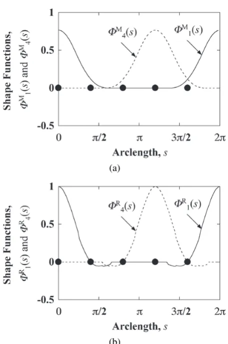
Let us investigate the behavior of the MLS shape func-tions and that of the RPIM one. In the numerical experi-ments, five nodes are uniformly placed on the boundary of a unit circle. In the MLS shape function, the spline-type weight function is assumed. The explicit form of the weight function is given by

wi(s)=ω(|s−si|/Ri),

(a)

(b)

Fig. 1 (a) The behavior of the MLS shape functions and (b) that of the RPIM shape function. Here, the parameters are fixed as follows:m=2 andγ=1.6. The symbol• indi-cates the boundary node.

In the RPIM shape function,ri(s) is given by the compactly

supported radial basis function (CSRBF) [8] and its ex-plicit form is expressed as

ri(s)=ρ(|s−si|/Ri),

ρ(r)=(1−r)3(3r+1).

In both shape functions,Riis defined by

Ri=γmin smod (i+1,N)−si , smod (i−1,N)−si ,

whereγis a constant.

As a typical example, we compute the shape functions, ΦM

i (s) and ΦRi(s), and show their behavior

(Figs. 1 (a) and 1 (b)). We see from these figures that both shape functions are a smooth function with a period of 2π. Moreover, the MLS shape function lacks the Kronecker delta function property, whereas the RPIM shape function satisfies it.

From these results, we can completely remove the de-merit of the MLS approximation by using the RPIM ap-proximation.

3. Performance Evaluation

In this section, the performance of the X-BNM with

Table 1 Evaluation Environment.

Parameter Value

OS MacOS X 10.9

CPU Intel Core i5 1.3 GHz

Memory 4 GB

Compiler gfortran 4.8.2 Compiler option -O3

the periodic RPIM shape function is investigated numeri-cally. As an example problem, we adopt the 2-D Poisson problem over Ω ≡

(x,y) x−Δ(y/2)22+(y/2)2<1

and the given functions used in the 2-D Poisson prob-lem are determined so that the analytic solution may be

u =e−3(x2_+y2₎

−coshxsiny+cosxsinhy. Also, only the Direclet problem is solved throughout the present study.

When the Poisson equation is transformed to an equiv-alent boundary integral equation, the equation contains not only the boundary integrals but also a domain integral. In order to remain only the boundary integrals, we assume that the right hand sideg(x) of the Poisson equation is ap-proximated as

g(x)=

M

l=1

αlρ

⎛ ⎜⎜⎜⎜⎜ ⎝ x−_R¯xl

⎞ ⎟⎟⎟⎟⎟

⎠, (9)

wherex1,x2,· · ·,xM are poles on∂Ω∪Ω. Moreover, ¯R

andαl’s are all constants. Throughout the present study, ¯R

is fixed as ¯R=1.5.

The more detail with respect to the discretization of the 2-D Poisson problem by means of the X-BNM can be found in [3]. In the following, the Gauss-Legendre quadra-ture withNGis employed as the integration method and its

value is fixed asNG =12. Moreover, the evaluation

envi-ronment is shown in Table 1.

In our previous work, parameters used in the MLS shape function are fixed asm= 1 andγ =1 [3]. Hence, we employ parameters of the RPIM shape function as is the case in the MLS shape function.

As the measure of the accuracy, we adopt the relative error defined by

ε=

_u

A−uN 2

+qA−qN 2

_u

A 2

+qA 2 ,

where the subscript notations, A and N, are analytic and numerical solutions, respectively, and denotes the Euclidean norm. In this section, the X-BNM with the MLS shape function, the X-BNM with the conventional RPIM shape function and the X-BNM with the periodic RPIM shape function are called the X-BNM(MLS), the X-BNM(Conventional RPIM) and the X-BNM(Periodic RPIM), respectively.

Fig. 2 Dependence of the relative errorε on the the number N of boundary nodes for the case with Δ = 0. Here,

the symbols,, anddenote the X-BNM(MLS), the

X-BNM(Conventional RPIM) and the X-BNM(Periodic RPIM), respectively.

Fig. 3 Dependence of the approximation accuracy of (9) on the the numberMof poles for the case withΔ =0.

as a function of N and are depicted in Fig. 2. We see from this figure that the accuracy of the X-BNM(Periodic RPIM) is higher than that of the X-BNM(Conventional RPIM). Moreover, the accuracy of the X-BNM(Periodic RPIM) is almost equal to that of the X-BNM(MLS). In addition, the relative errors of the X-BNM(MLS) and the X-BNM(Periodic RPIM) are saturated forN500. In or-der to investigate this tendency in detail, we indicate the dependence of the approximation accuracy ofg(x) on the numberMof the poles. As the measure of the approxima-tion accuracy ofg(x), we adopt the relative error defined by

εg=

g(x)−

M

l=1

αlρ

⎛ ⎜⎜⎜⎜⎜ ⎝ x−_R¯xl

⎞ ⎟⎟⎟⎟⎟ ⎠

∞ g(x)_∞ ,

where _∞denotes the maximum norm. The relative er-ror εg is plotted as a function of M in Fig. 3. The

rel-ative error decreases with an increase in M, whereas it

Fig. 4 Dependence of the CPU timeτ on the the number N

of boundary nodes for the case with Δ = 0. Here,

the symbols,,anddenote the X-BNM(MLS), the

X-BNM(Conventional RPIM) and the X-BNM(Periodic RPIM), respectively.

Fig. 5 Dependence of the relative errorεon the triangularityΔ for the case withN=500. Here, the symbols,,and

denote the X-BNM(MLS), the X-BNM(Conventional

RPIM) and the X-BNM(Periodic RPIM), respectively.

almost becomes dominant with an increase in M for the case withM 700. This result shows that the limit ofεg

is almost equal to 10−4. Therefore, relative errors of the X-BNM(MLS) and the X-BNM(Periodic RPIM) become constant for N 500 because the discretization error is smaller than the approximation error ofg(x).

Next, we evaluate the speed of the X-BNM(Periodic RPIM). The CPU times are plotted as a function of N

in Fig. 4. This figure indicates that not only the speed of the X-BNM(Conventional RPIM) but also that of the BNM(Periodic RPIM) is faster than that of the X-BNM(MLS) for the case withN500.

RPIM) increase with an increase in Δ. However, both the relative error of the X-BNM(Periodic RPIM) and that of the BNM(MLS) are much lower than that of the X-BNM(Conventional RPIM) regardless ofΔ.

4. Conclusion

We have proposed the X-BNM with the periodic RPIM shape function so that the number of unknowns be-comes equal to that of boundary nodes (i.e., the shape func-tion has the Kronecker delta funcfunc-tion property). In ad-dition, its performance has been investigated numerically. Conclusions obtained in this paper are summarized as fol-lows.

1. The accuracy of the X-BNM with the periodic RPIM shape function is almost equal to that with the MLS shape function. Even if the boundary shape is strongly concave, this tendency does not change. 2. The speed of the X-BNM with the periodic shape

function is always faster than that with the MLS shape function for the case where the number of boundary nodes exceeds a certain limit.

From the above mentions, we might conclude that the X-BNM with the periodic RPIM shape function is a powerful method for a large-scale simulation. In the future work, we will apply the X-BNM with the periodic RPIM shape function to the problems of the field of the nuclear fusion

science such as the boundary-value problem of the Grad-Shafranov equation.

Acknowledgement

This work was supported in part by Japan Society for the Promotion of Science under a Grant-in-Aid for Scien-tific Research (C) No. 24560321 and a Grant-in-Aid for Young Scientists (B) No. 25870630. In addition, a part of this work was also performed with the support and under the auspices of the NIFS Collaboration Research program (NIFS13KNTS025, NIFS13KNXN267).

[1] M. Itagaki and T. Fukunaga, Eng. Anal. Bound. Elem. 30, 746 (2006).

[2] Y.X. Mukherjee and S. Mukherjee, Int. J. Numer. Meth. Eng.

40, 797 (1997).

[3] A. Saitoh, S. Nakata, S. Tanaka and A. Kamitani, Informa-tion12(5), 973 (2009) [in Japanese].

[4] A. Saitoh, N. Matsui, T. Itoh and A. Kamitani, IEEE Trans. Magn.47(5), 1222 (2011).

[5] A. Saitoh, K. Miyashita, T. Itoh, A. Kamitani, T. Isokawa, N. Kamiura and N. Matsui, IEEE Trans. Magn.49(5), 1601 (2013).

[6] J.G. Wang and G.R. Liu, Int. J. Numer. Meth. Eng.54(11), 1623 (2002).

[7] A. Saitoh, T. Itoh, N. Matsui and A. Kamitani, IEEE Trans. Magn.50(2), 7011404 (2014).