doi: 10.11648/j.acis.20130103.11
Application of fuzzy logic to multi-objective scheduling
problems in robotic flexible assembly cells
Khalid Abd
1, 2, *, Kazem Abhary
1, Romeo Marian
11School of Engineering, University of South Australia, Mawson Lakes 5095, South Australia 2School of Industrial Engineering, University of Technology, Baghdad, Iraq
Email address:
[email protected](K. Abd), [email protected](K. Abhary), [email protected](R. Marian)
To cite this article:
Khalid Abd, Kazem Abhary, Romeo Marian. Application of Fuzzy Logic to Multi-Objective Scheduling Problems in Robotic Flexible Assembly Cells. Automation, Control and Intelligent Systems. Vol. 1, No. 3, 2013, pp. 34-41. doi: 10.11648/j.acis.20130103.11
Abstract:
This paper is aimed at developing a methodology to solve a multi-objective problem in robotic flexible assembly cells. The proposed methodology is based on three main steps: (1) scheduling of the RFACs using different common rules, (2) normalisation of the scheduling outcomes, and (3) selection of the optimal scheduling rules, using a fuzzy inference system. In this paper, four rules, namely short processing time, long processing time, earlier due date and random, are examined. Four objectives are considered simultaneously: scheduling length, total transportation time, utilisation rate and workload rate. A realistic case study is provided for demonstrating applicability of the suggested methodology. The results show that the methodology is practical and works in RFACs settings.Keywords:
Assembly Cells, Scheduling Rules, Fuzzy Logic, Robotics1. Introduction
Flexible manufacturing systems have attracted significant attention in recent years, due to their flexibility and dexterity in dealing with unexpected events. One class of such systems is called robotic flexible assembly cells (RFACs). RFACs are highly modern systems, structured with industrial robot(s), assembly stations and an automated material handling system, all monitored by computer numerical control [1-3].
The design of RFACs with multi robots leads to increased productivity in a shorter cycle time and with lower production costs [4]. However, there are certain difficulties that have arisen with this design concept. For example, more than one robot operating simultaneously in the same work environment requires a complex control system to prevent collisions between robots [5], and also to prevent deadlock problems [6]. Moreover, industrial robots must be employed as effectively as possible due to the high cost of the robots [4]. To overcome the above difficulties, efficient scheduling of RFACs is required.
Few studies have been devoted to scheduling RFACs [7]. These studies may be categorised according to the approaches adopted. In the first category are those studies which applied heuristic approaches to solve scheduling problems such as Lee and Lee [6], Nof and Drezner [8], Lin
et al. [9], Pelagagge et al. [10], Sawik [11], Jiang et al. [12] and Rabinowitz et al. [13]. The studies in the second category investigated simulation as an approach to scheduling RFACs, for instance, Gilbert et al. [14], Hsu and Fu [15] and Barral et al. [16]. There are only two studies in the third category, by Brussel et al. [17] and Dell Valle and Camacho [18], which implemented expert systems approaches to solve scheduling problems. The major limitation of the above studies is that they concentrated on assembly of only one type of product at a time.
In our previous study [19], scheduling RFACs for concurrent assembly of multi-products was proposed. Different scheduling rules were implemented. The results showed that making a decision on the best scheduling rule based on multi criteria is a considerably complex task. This study does not address how to select the most suitable scheduling rule.
2. Fuzzy Logic
Fuzzy Logic (FL) was first introduced by Zadeh in 1965 [21]. FL is a nonlinear mapping of an input data vector into a scalar output. A fuzzy inference system (FIS) consists of four components [22, 23]:
• Fuzzification: In this interface, the real world variables (crisp input data) are converting into linguistic variables (fuzzy values). This step can be done using the membership functions of input variables.
• Knowledge base: In this component, the membership functions are determined. These membership functions reflect a human reasoning mechanism.
• Inference engine: In this component, fuzzy input values convert to fuzzy output using IF-THEN type fuzzy rules. These rules reflect human experts’ knowledge of the system. The number of decision rules depends on the number of input variables and their linguistic values.
• Defuzzification: In this interface, the fuzzy outputs are translates into a crisp value. The defuzzification process can be achieved using the membership functions of output variable. Several methods have been proposed for defuzzification process. The well-known method for defuzzification process, named centre of gravity (COG) [23, 24] is used to transform the fuzzy inference output into non-fuzzy value.
The important component in a FIS is the knowledge base. This component stores both the membership functions and the IF-THEN rules base provided by experts. Three steps, linguistic variables, membership functions and fuzzy rules, are prepared to establish a knowledge base [25, 26]. The next sub section will describe these three steps.
2.1. Linguistic Variables
A linguistic variable is the procedure to describe variables in terms of words instead of their values. A linguistic variable consists of a set of terms called linguistic terms, denoted by T. For example, if processing time is interpreted as a linguistic variable, terms such as “Low”, “Medium” and “High” are used in a real industry context. Hence, a linguistic variable of processing time could be T
[processing time] = [Low, Medium, High].
2.2. Membership Functions
A membership function (MF) embodies a fuzzy set à graphically. The values of the membership functions are between 0 and 1, denoted by µÃ (x) where x is an element of Ã; these values are called degrees of membership.
2.3. Fuzzy Rule
A fuzzy rule is structured to control the output variable. These rules can be provided by experts or may be extracted from numerical data. A fuzzy rule has two parts, the
antecedent and the consequent: IF <antecedent> THEN <consequent>. For instance, IF x is A THEN y is B; where x
and y are variables and A and B are linguistic variables.
3. Proposed Methodology
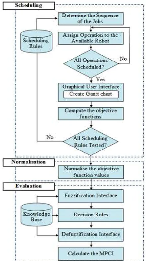
In this section, the architecture of the proposed methodology is presented. The methodology has three main steps: scheduling, normalisation and evaluation, as shown in Figure 1. The next sub sections will present these steps in detail.
Figure 1.Proposed methodology for scheduling problems in RFACs
3.1. Scheduling
• Short Processing Time (SPT): select job with minimum processing time first.
• Long Processing Time (LPT): select job with maximum processing time first.
• Random (RAND): jobs are sequenced randomly.
• Earlier Due Date (EDD): jobs are sequenced according to their due dates.
Four objective functions are considered to evaluate the scheduling. The mathematical expressions of these objectives were formulated in our previous study [19].
• Scheduling length (Tmax): One of the common
objective functions in scheduling is called scheduling length or cycle time. Tmax represents the maximum
total completion time performed by the robot. Total Transportation Time (Ttran): The sum time required to
travel the robot between cell resources to finish assembly of products. Ttran aims at measuring the
amount of movement of each robot in RFACs, during one cycle time.
• Utilisation rate (UR): Another important objective
function, that gives a clear perception as to whether the robots are used efficiently.
• Workload rate (WR): WR is a measure of RFAC
balance.
In this study, six assumptions are considered. First, the optimum assembly sequence of each product is given in advance. Second, each product uses some or all of the cell resources. Third, each robot can perform only one task at a time. Fourth, no interruptions such as resources breakdown occur in the cell. Fifth, the processing time of each task is deterministic and is known in advance. Sixth, the set-up times are assumed done when the cell is off-line, so not considered.
3.1. Normalisation of the Objective Values
This is done by converting the objectives functions values to range between 0 and 1. This process is called normalisation. In this study, two objective functions, Tmax
and Ttran, are to be minimised, and the other objective
functions, UR and WR, are to be maximised. Therefore, the
normalisation can be done using the following two equations, where ƞi(k) denotes the value of objective function k in
scheduling rule i. The equation (1) is for the objective functions to be maximised, while the equation (2) is for the objective functions to be minimised.
µ , 0 µ 1 (1)
According to the equation (1), it can be seen that the rule i
with minimum value of objective function k has a normalised value of 1 and the rule i with maximum value of objective function k has a normalised value equal to 0.
µ , 0 µ 1 2
From the equation (2), it can be concluded that the rule i
with minimum value of objective function k has a normalised value of 0 and the rule i with maximum value of objective function k has a normalised value of 1.
Therefore, the scheduling rule with low Tmax, low Ttran,
high UR and high WR will take high rank. 3.3. Evaluation of Scheduling Rules using FIS
In order to find out the optimum scheduling rule for multiobjective problems in RFACs, FIS is used. For a single objective, the optimum scheduling rule is the one having the highest normalisation value. Multi-objective function optimisation is not as straightforward as that of a single objective function optimisation. To overcome this problem, a multiple performance characteristics index (MPCI) based FIS is developed to derive the optimal solution.
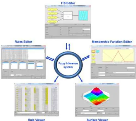
In this study, FIS is implemented using the MATLAB fuzzy toolbox. The fuzzy logic toolbox consists of five graphical user interface tools (GUIs) for building, editing and observing any fuzzy inference system [27, 28]. These tools are: the fuzzy inference system (FIS) editor, the membership function editor, the rule editor, the rule viewer, and the surface viewer, as shown in Figure 2. The GUIs are dynamically connected, and the altering of any GUI can affect the other GUIs.
Figure 2. Fuzzy inference system and its integral components in MATLAB software
3.3.1. FIS Editor
The FIS editor handles the information related to the variables of inputs and output, such as variables' names and their numbers. In the present study, The FIS contains four input parameters and one output parameter. The input parameters are the normalisation of Tmax, Ttran, UR and WR,
while MPCI is the output parameter.
The Tmax, Ttran, UR and WR are break down into a set of
very large (VL) and huge (H). Table 1 shows the different linguistic values of the inputs/output and their numerical range.
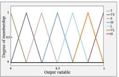
3.3.2. Membership Function Editor
The membership function editor is used to construct the shapes of all the input/output parameters. There are different types of membership functions’ shapes such as triangular, trapezoidal, Gaussian, singleton, etc. The triangular shape is the common membership functions shape and a powerful way to approach the convex function [29]. In this study, the membership functions for inputs/output are plotted using the triangular shape, shown in Figures 3 and 4 respectively.
Table 1. Input and output variables with their fuzzy values.
System variables
Linguistic variables
Linguistic
Value Numerical Range
Inputs Tmax,Ttran,
UR and WR Low
Medium
High
[0– 0.25]
[0.25–0.75]
[0.75–1]
Outputs MPCI
Tiny
Very Small
Small
Medium
Large
Very Large
Huge
[0– 0.167]
[0– 0.334]
[0.167 – 0.5]
[0.334 – 0.66]
[0.5 – 0.834]
[0.667 – 1]
[0.834 –1]
Figure 3. Membership functions for fuzzy input variables
Figure 4. Membership functions for fuzzy output variable
3.3.3. Rule Editor
The rule editor is for editing the list of fuzzy rules that are used to control the output variable. The fuzzy rule is constructed based on the number of linguistic variables for inputs/output. In the present study, to control the output parameter (MPCI), fuzzy rules are structured. Fuzzy rules are derived directly based on the formula (nm), where nand denote input parameters and their linguistic values. Thus, the number of fuzzy rules is 43 = 64. Each rule is mathematically evaluated through a process named implication. In this study, Mamdani implication is applied [30].
The generic form of a fuzzy rule can be stated in the following form: IF (Tmax is ■) and (Ttran is ■) and (UR is ■)
and (WR is ■) THEN (MPCI is ■). The black boxes represent
the linguistic variables for each of the fuzzy variables. Example of the fuzzy rules derived is shown in the examples below.
1. IF (Tmax is Low) and (Ttran is Low) and (UR is High) and
(WR is High) THEN (MPCI is Huge).
2. IF (Tmax is Medium) and (Ttran is Low) and (UR is High)
and (WR is High) THEN (MPCI is Very Large).
3. IF (Tmax is High) and (Ttran is Low) and (UR is High)
and (WR is High) THEN (MPCI is Large).
. .
64. IF (Tmax is High) and (Ttran is High) and (UR is Low)
and (WR is Low) THEN (MPCI is Tiny). 3.3.4. Surface Viewer
The surface viewer allows the user to visualize the relation between input fuzzy variables and the output of a fuzzy system in a three-dimensional graph, the X-axis and Y-axis in the 3D graph represent any two selected input variables, and the Z-axis represents the output of a fuzzy system. In this study, since the number of input variables is four, the number of generated 3D graphs is six.
3.3.5. Rule Viewer
The rule viewer displays a graphical representation of the values of the input variables and the output of a fuzzy system, through all the fuzzy rules.
4. Case Study
The illustration of the proposed approach is demonstrated using a realistic case study. The multi robot assembly cell consist of two robots (R1 and R2) that can use
a number of tools that can be changed in a tool magazine (GC), assembly stations (AS1, AS2, AS3, AS4& AS5) where
components are assembled, transfer table (TT) to transfer partial assemblies from one robot to another. There are also two conveyors. The first one (IC) supplies components to the cell and the second one (OC) is for conveying out a final product when assembly processes are completed, as shown in Figure 5.
robot arms cannot move from one place to another directly. The reason for this is to avoid collision with the other robot arms. This is achieved by assigning control points
, , … , to simplify path planning and avoid collision.
Second, to prevent collisions between robots in a shared area, more than one robot cannot access the same resource simultaneously. Third, to fetch and assemble parts, the hand of each robot should be equipped with the right tool; however, a specific tool may not be available for the two robots concurrently, due to the restricted number of available tools [19].
Figure 5. Robotic flexible assembly cells
Assume that three sizes of supply tanks are to be assembled in the RFACs presented as shown in Figure 6. The tanks are, essentially, chambers of constant level which supply, through gravity, liquid fuel for burners. They are composed of 13, 15 and 31 parts, respectively.
For manipulation within the cell, the tanks are loaded on a pallet that requires a gripper G1 (to be used for T1, T2 and T3),
whereas for the lids, a second pallet is utilised, requiring another gripper G2 (for L1, L2 and L3). The grippers are
interchangeable. Each robot can work with either G1 or G2, as required. The times needed to perform tool change operations are shown in Table 3. Table 4 shows the time
required to move the robot between two positions in the cell.
Figure 6. Exploded view of supply tanks 11, 21 and 51
Further, assume that RFACs do not have to be stopped to load the AS with consumables like fasteners, parts and sealants (a realistic assumption for modern assembly machines with magazines of parts and components). The
Assembly stations in the RFACs are dedicated to the specific assembly operations, as shown in Table 2. This table also gives details of description for each assembly operations.
Table 2. Assembly operations requirements
Description Station Operation times Tank 11 Tank21 Tank51
Sealant on Tank AS1 5 10 18
Assemble Lid AS2 5 5 5
Insert screws M6x16 AS2 8 12 20
Sealant on Lid AS1 5 5 10
Fit the Level Control unit AS3 5 5 10
Fit the Safety Valve AS4 0 0 5
Insert screws M3x12 AS2 8 8 24
Assemble Inlet & Outlet AS5 10 10 20
Total processing time (Sec.) 46 55 112
Due date (Sec.) 250 200 300
Table 3. Tool change requirements
Tool name Number of
available tools Part assignment
Tool change time (s)
Gripper 1 2 T1, T2, T3 3
Gripper 2 1 L1, L2, L3 3
Table 4. Transportation time for robots between cell resources
Path description Position Time (s)
Robot move from resource to control point
AS1,2,3/GC/TT C1,2
AS2,4,5/GC/TT C3,4 1
Robot move from control point to resource
C1,2 AS1,2,3/GC/TT
C3,4 AS2,4,5/GC/TT 2
Robot move between control point and conveyor
C1, C3 IC
C2, C4 OC 1.5
Robot move between two control points
C1 C2
C3 C4 1
Robot move directly from station to another
AS1 AS3
AS4 AS5 2
5. Results and Discussion
In order to examine the effectiveness of the proposed methodology, four experiments are executed. Each experiment is performed with different scheduling rules. These rules are used to generate the sequence of job flow to the RFACs. Table 5 shows the list of scheduling rules adopted in this study.
Table 5. List of dispatching rules and the priority of the jobs
NO Scheduling Rule Sequence
A Short Processing Time (SPT) Tank11 Tank21 Tank51
B Long Processing Time (LPT) Tank51 Tank21 Tank11
C Due date (DD) Tank21 Tank11 Tank51
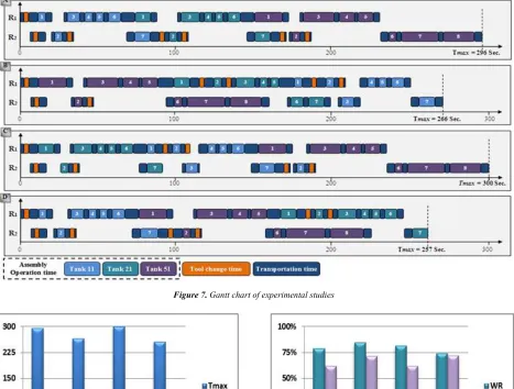
Figure 7 illustrates the Gantt chart of the final schedule produced by different rules. The results of the overall objective functions of the four scheduling rules are presented in Figure 8. Figure 8(a) shows the Tmax and Ttran
results of the scheduling rules. From this figure it can be
seen that the SPT and RAND obtain the best results for minimising the Ttran and Tmax respectively compared with the
other scheduling rules. LPT and EDD are the worst in minimising the Ttran and Tmax respectively.
Figure 7. Gantt chart of experimental studies
Figure 8. Experimental results for scheduling rules
Figure 8(b) shows the UR and WR results of scheduling
rules. In this figure, LPT emerges as the best rule among all four scheduling rules for maximising the WR; EDD ranks
second, and still obtains good results among all the other selected rules from the previous literature. RAND appears to be the worst rule for maximising the WR. RAND emerges as
the best rule among all four rules for maximising the UR,
followed by LPT, EDD and SPT. Depending on the previous results, making a decision of the best scheduling rule based on one objective function is simple; nevertheless determination of the optimal scheduling through
consideration of multi objective functions is a considerably more complex task. The next step of the proposed methodology is normalisation of the objective functions’ values. The ranges of values for the four objective functions,
Tmax, Ttran, UR and WR are all different. To avoid the different
ranges, the values must be normalised to values between 0 and 1. In this case, since the objective of Tmax and Ttran is
minimising, and the objective of UR and WR is maximising,
After the objective functions’ values are normalised, MPCI is calculated to derive the optimal scheduling rule. The MPCI calculation can be done using FIS. The fuzzy logic toolbox in MATLAB is used to construct the FIS of the MPCI. In this study, since the number of input parameters is four, the number of generated 3D graphs is six. Figure10 illustrates one example of a 3D graph. In this Figure, the MPCI resulting from the interaction of Tmax and Ttran is
shown. It can be seen that the low Tmax and Ttran values give a
high score of MPCI. Moreover, it can be concluded that the
Tmax has a higher influence than the Ttran on the MPCI.
Figure 9. Normalisation of the objective functions’ values
Figure 10. Surface analysis between inputs/output combinations
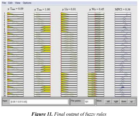
The rule viewer, which displays a graphical representation of the values of the input parameters and the output of a fuzzy system through all the fuzzy rules, is shown as an example in Figure 11. This figure shows the rule viewer for MPCI, which can accept any value of four input parameters:
Tmax, Ttran, UR and WR. The output (MPCI) in this Figure can
be interpreted easily, as for example, as in the following: IF
Tmax is (0.09), Ttran is (1.00), the URis (0.01) and WR is (0.45)
THEN MCPI will be (0.36).
Table 6 shows the MPCI values corresponding to each experimental run obtained by using the FIS. LPT gives the highest MPCI value among the four rules; EDD is the worst one on this numerical example. The final ranking of the scheduling rules is LPT – RAND – SPT – EDD in descending order of preference.
Figure 11. Final output of fuzzy rules
Table 6. List of dispatching rules and the priority of the jobs
Scheduling Rule µ Tmax µ Ttran µ UR µ WR MPCI
SPT 0.09 1.00 0.01 0.45 0.36
LPT 0.79 0.00 0.93 1.00 0.71
EDD 0.00 0.67 0.00 0.72 0.33
RAND 1.00 0.75 1.00 0.00 0.61
6. Conclusion
This paper has dealt with the problem of scheduling RFACs with consideration of assemble multi-product, under different experiments. These experiments were performed using four scheduling rules: SPT, LPT, EDD and RAND. The scheduling results showed that the decision making of selecting the best rule based on one objective function is a simple way; nevertheless determination of the optimal scheduling rule through consideration of multi-objective functions is a considerably more complex task. Consequently, in this paper, FIS is developed to select the optimal rule for scheduling RFACs; to minimise the scheduling length (Tmax) and total transportation Time (Ttran);
and to maximise of the utilisation rate (UR) and workload
rate (WR). The FIS results showed that fuzzy logic is a
powerful technique and easy to use for handling the multi objective optimisation problem. The proposed methodology is implemented using only four scheduling rules. This study could be extended to include other types of rules such as critical ratio (CR) and minimise slack time (MST). A possible extension would be development of a new rule for scheduling RFACs, by combine all input variables such as processing time, due date and batch size in one rule; and comparing the results that are obtained by the new rule with the common rules.
References
assembly cell using a dynamic knowledge base", IEEE transactions on systems, man, and cybernetics, vol. 23, pp. 766-782, 1993.
[2] T. Sawik, “Production planning and scheduling in flexible assembly systems” Springer -Verlag, Berlin, 1999.
[3] R. M. Marian, A. Kargas, L. H. S. Luong, and K. Abhary, "A framework to planning robotic flexible assembly cells", presented at the 32nd International Conference on Computers and Industrial Engineering, Limerick, Ireland, 2003. [4] E. K. Xidias, P. T. Zacharia, and N. A. Aspragathos, "Time
optimal task scheduling for two-robotic manipulators operating in a three-dimensional environments", Journal of Systems and Control Engineering, vol. 224, pp. 845-855, 2010.
[5] S. Y. Nof and J. Chen, "Assembly and disassembly: an overview and framework for cooperation requirement planning with conflict resolution", Journal of Intelligent and Robotic Systems vol. 37, pp. 307–320, 2003.
[6] J.-K. Lee and T.-E. Lee, "Automata-based supervisory control logic design for a multi-robot assembly cell", International Journal Computer Integrated Manufacturing, vol. 15, pp. 319-334, 2002.
[7] K. Abd, K. Abhary, and R. Marian, "A scheduling framework for robotic flexible assembly cells", AIJSTPME-Asian International Journal of Science and Technology in Production and Manufacturing Engineering, vol. 4, pp. 30-37, 2011.
[8] S. Y. Nof and Z. Drezner, "The multiple-robot assembly plan problem", Journal of Intelligent and Robotic Systems vol. 7, pp. 57-71, 1993.
[9] H. C. Lin, P. J. Egbelu, and C. T. Wu, "A two-robot printed circuit board assembly system", International Journal of Computer Integrated Manufacturing, vol. 8, 1995.
[10] P. M. Pelagagge, G. Cardarelli, and M. Palumbo, "Design criteria for cooperating robots assembly cells", Journal of Manufacturing Systems, vol. 14, pp. 219-229, 1995. [11] T. Sawik, "Integer programming models for the design and
balancing of flexible assembly systems", Mathematical and Computer Modelling vol. 21, pp. 1-12, 1995.
[12] K. Jiang, L. D. Seneviratne, and S. W. E. Earles, "Scheduling and compression for a multiple robot assembly work cell", production Planning & Control, vol. 9, pp. 143-154, 1998. [13] G. Rabinowitz, A. Mehrez, and S. Samaddar., "A scheduling
model for multi-robot assembly cells", International Journal of Flexible Manufacturing Systems vol. 3, pp. 149-180 1991. [14] P. R. Glibert, D. Coupez, Y. M. Peng, and A. Delchambre, "Scheduling of a multi-robot assembly cell", Computer Integrated Manufacturing Systems, vol. 3, pp. 236-245, 1990. [15] H. Hsu and L. C. Fu, "Fully automated robotic assembly cell:
scheduling and simulation", presented at the IEEE International Conference on Robotics and Automation, National Taiwan University, 1995.
[16] D. Barral, J.-P. Perrin, and E. Dombre, "Flexible agent-based robotic assembly cell", New Mexico, 1997.
[17] H. Van Brussel, F. Cottrez, and P. Valckenaers, "SESFAC: A scheduling expert system for flexible assembly cell", Annals of The CIRP, vol. 39, pp. 19-23, 1990.
[18] C. Del Valle and E. F. Camacho, "Automatic assembly task assignment for a multi robot environment", Control engineering practice, vol. 4, pp. 915-921, 1996.
[19] K. Abd, K. Abhary, and R. Marian, "Scheduling and performance evaluation of robotic flexible assembly cells under different dispatching rules", Advances in Mechanical Engineering, vol. 1, 2011.
[20] K. Abd, K. Abhary, and R. Marian, "An MCDM Approach to Selection Scheduling Rule in Robotic Flexible Assembly Cells", presented at the International Conference on Mechanical, Aeronautical and Manufacturing Engineering, Venice, Italy, 2011.
[21] L. A. Zadeh, "Fuzzy sets", Information and Control, vol. 8, pp. 338-353, 1965.
[22] L. A. Zadeh, "Fuzzy-algorithm approach to the definition of complex or imprecise concept", International Journal of Manachines Studies, vol. 8, pp. 249–291, 1976.
[23] J. M. Mendel, "Fuzzy logic systems for engineering: A tutorial", Proceedings of the IEEE 83 pp. 345–377, 1992. [24] J. Yen, R. Langari, “Fuzzy logic intelligence, Control, and
Information”, Prentice Hall Publishing Company, 1999. [25] K. Abd, K. Abhary, and R. Marian, "Intelligent modeling of
scheduling robotic flexible assembly cells using fuzzy logic", presented at the 12th WSEAS International Conference on Robotics, Control and Manufacturing Technology, Rovaniemi, Finland, 2012.
[26] K. Abd, K. Abhary, and R. Marian, "Efficient scheduling rule for robotic flexible assembly cells based on fuzzy approach", presented at the 45th CIRP Conference on Manufacturing Systems, 2102.
[27] Mathworks 2009. “Fuzzy logic toolbox user’s guide”, http://www.mathworks.com/access/helpdesk/help/pdf_doc/f uzzy/fuzzy.pdf.
[28] S. N., Sivanandam, S. Sumathi, and S. N. Deepa, “Introduction to fuzzy logic using MATLAB”, New York, Springer, 2007.
[29] W. Pedrycz, "Why triangular membership functions?” Fuzzy Sets and Systems pp. 21–30, 1994.