Minimization of Unconstrained Nonpolynomial Large-Scale Optimization Problems Using Conjugate Gradient Method Via Exact Line Search

http://www.sciencepublishinggroup.com/j/ajmme doi: 10.11648/j.ajmme.20170101.13

Minimization of Unconstrained Nonpolynomial Large-Scale

Optimization Problems Using Conjugate Gradient Method

Via Exact Line Search

Adam Ajimoti

1

, Onah David Ogwumu

2

1

Department of Mathematics, University of Ilorin, Ilorin, Nigeria 2

Department of Mathematics, Federal University Wukari, Wukari, Nigeria

Email address:

[email protected] (A. Ajimoti), [email protected] (O. D. Ogwumu)

To cite this article:

Adam Ajimoti, Onah David Ogwumu. Minimization of Unconstrained Nonpolynomial Large-Scale Optimization Problems Using Conjugate Gradient Method Via Exact Line Search. American Journal of Mechanical and Materials Engineering. Vol. 1, No. 1, 2017, pp. 10-14. doi: 10.11648/j.ajmme.20170101.13

Received: February 28, 2017; Accepted: March 22, 2017; Published: April 7, 2017

Abstract:

The nonlinear conjugate gradient method is an effective iterative method for solving large-scale optimization problems using the iterative scheme x(k+1)= x(k)+ αkd(k) where: x(k+1) is the new iterative point, x(k) is the current iterative point, αk is the step-size and d(k) is the descent direction. In this research work, we employed the technique of exact line search to

compute the step-size in the iterative scheme mentioned above. The line search technique gave good results when applied to some non-polynomial unconstrained optimization problems.

Keywords:

Iterative Point, Non Polynomial, Unconstrained Optimization, Conjugate Gradient Method, Descent Direction,

Exact Line Search, Iterative Scheme

1. Introduction

We wish to consider recent developments in large-scale unconstrained optimization. We would like to state however that small-scale optimization remains an active area of research, and that advances in this field often translate into new algorithms for large-scale problems.

The problem under consideration is:

min ( ), n

f x x∈R (1)

where f is a smooth function of n variables. We assume that n is large, sayn>500,and we denote the gradient of f by g. An important recent development has been the appearance of effective tools for automatically computing the derivatives and for detecting partially separable structures. These programs are already having a significant impact in the practice of optimization and in the design of algorithms, and their influence is certain to grow with time.

We devote much attention to this topic because understanding the characteristics of the objective function is crucial in large-scale optimization.

1.1. Large-Scale Problems

We consider the problem of determining the value of a vector of decision variables x∈Rn that minimizes an objective function f R: n →R,when x is required to belong to a feasible set S⊆Rn, i.e. we consider the problem

min

x∈s f x( ) (2)

In this case we say the problem in equation (2) is unconstrained if S = Rn and when n is a large number, then the problem in equation (2) is called a large-scale problem.

1.2. Large-Scale Unconstrained Optimization Problems

Large-scale unconstrained optimization problems do arise in many sectors such as in:

(i) Energy (optimal plant operations, revenue and risk management, and strategic pricing).

(ii) Finance (option pricing, demand optimization and nonlinear least-squares data fitting).

distribution networks).

(iv) Marketing (quantitative marketing). (v) Economics (computational economics).

(vi) Manufacturing (CAD, optimal computer chip layout, and transportation network).

(vii)Mining, etc.

1.3. Methods of Solution

Several algorithms have been developed for solution of large-scale problems by different type of methods. The methods are Newton's method, quasi-Newton method, conjugate gradient method, etc.

1.3.1. Newton Method

This is the most powerful algorithm for solving large-scale nonlinear optimization problems. It normally requires the fewest number of function evaluations, is very good at ill-conditioning, and is capable of giving the most accurate answers. It may not always require the least computing time, this depends on the characteristics of the problem and the implementation of the Newton iteration but it represents the most reliable method for solving large-scale problems. Newton's method is well known and widely used to find zeroes of differentiable functions. Sufficiently close to a zero, it converges very rapidly but the convergence is not guarantee because it requires large computing storage space.

1.3.2. Quasi-Newton Method

There have been various attempts to extend the quasi-Newton updating to the large-scale case, and two of them have proved to be very successful in different contexts. The first idea consists of exploiting the structure of partially separable functions by updating approximations to the Hessians of the interval functions. This gives rise to a powerful algorithm of wide applicability, and whose only drawback is the need to fully specify a partially separable representation of the function. The second approach is that of limited memory updating in which only a few vectors are kept to represent the quasi-Newton approximation to the Hessian. They are not as robust and as rapidly convergent as partially separable quasi-Newton methods, but are probably much more widely used.

1.3.3. Conjugate Gradient Method

It has been shown that any minimization method that makes use of the conjugate directions is quadratically convergent. This property of quadratic convergence is very useful because it ensures that the method will minimize a quadratic function in n steps or less. Since any general function can be approximated reasonably well by a quadratic near the optimum point, any quadratically convergent method is expected to find the optimum point in a finite number of iterations.

We chose this particular method for the minimization of unconstrained non polynomial large-scale optimization problems. So, we will take this out to another section of this presentation in order to be able to describe more features

about the method.

2. Conjugate Gradient Method

The conjugate gradient method is a computational procedure for solving the unconstrained problem in equation (1). And the method has the following characteristics:

i. It solves quadratic problems of n variables in n steps. ii. It requires relatively small increase in computer time

per iteration and requires very low memory space. iii.It has a well worked-out theory.

All descent methods require the evaluation of the function and the gradient. We now give the following definition of the gradient of a function. The partial derivatives of a function f, with respect to each of n-variables are collectively called the gradient of the function and denoted by ∇f i.e,

1 2

( ) ( ) ( )

( ) ∂ ,∂ , ,∂ 

∇ = 

∂ ∂ ∂

 

…

T

n

f x f x f x

f x

x x x (3)

The gradient is an n-component vectors and it has a very important property that the gradient vector represents the direction of steepest ascent. In respect of this property, the negative of the gradient vector denotes the direction of steepest descent.

2.1. Conjugate Gradient Method for Non-Quadratic Functions

When the conjugate gradient method is used for minimizing non-quadratic functions, the method is known as non-quadratic CGM. The non-quadratic CGM generates the minimizing sequence (k)

{ x } starting with initial point x(0) using the iterative formula

(k 1) (k) (k)

x + =x + , =0,1, 2,…

Kd k

α

(4)

where αK is the step-length and

(k)

d is a search direction determined by

( ) ( 1)

( 1) ( )

, 0

, 1

+

+

_{− =}



=

− + ≥

 k k

k k

k

g k

d

g β d k (5)

In which g(k+1)is the gradient of f at

(k 1) x +

, i.e.,

( )

(k+1) _{= ∇} (k+1)

g f x (6)

and x(k+1) is a scalar known as the parameter of the method. The different formula for β_k indicate different CGMs. The following are the familiar βk’s available.

( 1)

( )

k T

HS k

k k T

k

g y

d y

β

+ =

2.Polak-Ribiere-Polyak [7]

( 1)

( ) ( )

k T

PRP k

k k T k

g y

g g

β

+ =

3.Fletcher-Reeves [4]

( 1) ( 1)

( ) ( )

k T k k FR

k k T k

g g

g g

β

+ +

=

4.Liu-Storey [10]

( 1) 1 ( ) ( )

k T

LS k

k k T k

g y

g d

β

+ + =

−

Where:

(+1) ( )

= k − k

k

y g g (7)

2.2. Algorithm for Non-Quadratic CGM

The steps involved in the implementation of a non-quadratic CGM are as stated below:

Step 1: Given x(0)∈Rn and ε >0 (small), set k = 0. If

( )k

g <ε, then stop, otherwise go to Step 2.

Step 2: Find

α

_k =arg min f x( ( )k +

α

d( )k ) ,

α

>0. Step 3: Update the variable x(k) and g(k) according to the equation (4) and (6) respectively. If g( )k <ε then stop, otherwise go to Step 4.

Step 4: Determine β_kfor the selected method and d(k) using the equation (5)

Step 5: Set k = k + 1, and go to Step 2.

3. Exact Line Search

This is the process of determining the value of the step-length α_k along the direction d(k) with the goal of ensuring convergence without deteriorating the rate of convergence. In this section, we consider the processes involved in finding the step-length α_k.

Given that f(x) is the objective function to be minimized using the CGM, the problem of finding α_k narrows down to finding the value

k

α =α which minimize

( ) (

( 1) ( ) ( )

)

( )

+ _{= + =}

k k k

f x f x αd f α (8)

for fixed values of x(k) and d(k). Since f(x(k+1)) becomes a function of only one variable, the method of finding αk involves one-dimensional minimization technique.

In every line search, the aim is to determine the value of the step-length αk >0 as stated above along the direction d(k) with the aim of ensuring con-vergence without deteriorating the rate of convergence. The first possibility of this is to set *

k

α =α with

( ) ( )

*

arg min ( )

= k + k

a f x αd (9) i.e, α_k is the value of α>0 that minimizes the function

f along the direction. d( )k.

α

*

in the equation (9) can be obtained by solving the equation

( ) ( )

( ) 0

∂ = + =

∂

k k

f

f x αd

α (10)

The technique employed in (10) yields an exact value

α

* and is referred to as an exact line search. Exact line search can be indirectly applied to non-polynomial objective functions on expansion using Taylor's series. Then the step-length αk can be obtained from the equation (10) by finding the real roots which satisfies the equation (9). This research work examines the computational process involved in implementing the exact line search for solving unconstrained optimization problems involving non-polynomial objective functions only.

4. Computational Details

4.1. Taylor's Series

Taylor's series expansion for a multivariable function f(x1,

x2,..., xn) is

2 3

1 1 1

( ) 1 ( ) 1 ( )

( ) ( ) ( ) ( ) ( )

2! 3!

n n n

i i i i i i

i i i i i i

f a f a f a f x f a x a x a x a

x x x

= = =

∂ ∂ ∂

= + − + − + −

∂ ∂ ∂

∑

∑

∑

⋯

4.2. Algorithm for Exact Line Search

Algorithm for exact line search as used in this work are stated below as follows:

Step 1: Given a non-polynomial objective function f(x), expand in Taylor's series and truncate the series after a number of terms.

Step 2: For the truncated f(x), substitute x with x + αd to get f(α).

i.e, f(α) = f(x + d) and write as a polynomial of α

Step 3: Compute the first-order derivative of f(x + αd) with

respect to α and equate to zero. i.e, f x( ) 0.

α

∂ ₌

∂

Step 4: Solve for the real root such that α > 0.

4.3. Computational Examples

The following non-polynomial functions obtained from Andrei [1] are used as computational examples

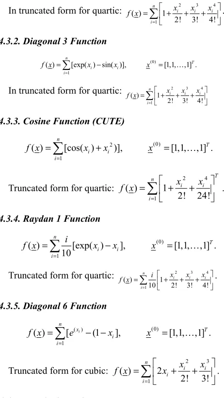
4.3.1. Raydan 2 Function

(0)

1

( ) [exp( ) ], [1,1, ,1] . n

T i i

i

f x x x x

=

In truncated form for quartic: 2 3 4

1 ( ) 1

2! 3! 4! n

i i i i

x x x

f x =   =  + + +   

∑

.

4.3.2. Diagonal 3 Function

(0)

1

( ) [exp( ) sin( )], [1,1, ,1] . n

T

i i

i

f x x x x

=

=

∑

− = …

In truncated form for quartic: 2 3 4 1

( ) 1

2! 3! 4!

n

i i i

i

x x x f x =   =  + + +   

∑

4.3.3. Cosine Function (CUTE)

(0) 2

1

( ) [cos( ) )], [1,1, ,1] .

n

T i i

i

f x x x x

=

=

∑

+ = …

Truncated form for quartic:

2 4

1

( ) 1

2! 24! T n i i i x x f x =   =  + +   

∑

.

4.3.4. Raydan 1 Function

(0)

1

( ) [exp( ) ], [1,1, ,1] .

10 n T i i i i

f x x x x

=

=

∑

− = …

Truncated form for quartic: 2 3 4 1

( ) 1

10 2! 3! 4!

n

i i i

i

x x x i f x =   =  + + +   

∑

.

4.3.5. Diagonal 6 Function

(0) ( )

1

( ) [ i (1 ], [1,1, ,1] .

n

x T

i i

f x e x x

=

=

∑

− − = …

Truncated form for cubic:

2 3

1

( ) 2

2! 3! n i i i i x x

f x x

=

 

=  + + 

 

∑

.

4.4. Numerical Results

The CGM Algorithm (2.2) was implemented using MATLAB 1.8.0347 [R2009a] codes on a HP laptop 620 with processor Pentium(R) Dual-Core CPU T4500 @2.30 GHz and RAM 2.00GB to solve the computational examples above. And the results obtained are tabulated in the tables below using the following notations:

n: (dimension)

ITR: (number of iterations)

f∗: (Optimal value of objective function f ) g∗ : (norm of the optimal gradient g ) Ext: (program execution time)

CE: (computational examples)

At: (average execution time per computation in each method)

Table 1. Numerical Result with PR.

CE n PR

(Dim) Itr f kg k Ext

4.3.1 5000 1 5.00e003 2.7e-011 0.07 10000 1 1.00e004 3.0e-011 0.09 4.3.2 5000 1 5.00e003 4.2e-012 0.02

10000 1 1.00e004 1.2e-011 0.02 At =

CE n PR

(Dim) Itr f kg k Ext

4.3.3 5000 1 5.00e003 9.1e-012 0.04 0.082 10000 1 1.00e004 1.7e-011 0.06 4.3.4 5000 1 1.56e010 4.3e-007 0.10 10000 3 5.005e010 6.0e-007 0.23

Table 2. Numerical Result with HS.

CE N HS

(Dim) Itr f kg k Ext

4.3.1 5000 1 5.00e003 2.7e-011 0.07 10000 1 1.00e004 3.0e-011 0.09 4.3.2 5000 1 5.00e003 4.2e-012 0.02 10000 1 1.00e004 1.2e-011 0.02

At =0.057 4.3.3 5000 1 5.00e003 9.1e-012 0.04

10000 1 1.00e004 1.7e-011 0.06 4.3.4 5000 1 1.56e010 4.3e-007 0.04 10000 3 5.005e010 6.0e-007 0.15 4.3.5 5000 1 -8.33e003 1.3e-013 0.05 10000 1 -1.67e004 1.8e-013 0.03

Table 3. Numerical Result with LS.

CE n LS

(Dim) Itr f kg k Ext

4.3.1 5000 1 5.00e003 2.7e-011 0.07 10000 1 1.00e004 3.0e-011 0.10 4.3.2 5000 1 5.00e003 4.2e-012 0.02 10000 1 1.00e004 1.2e-011 0.02

At = 0.055 4.3.3 5000 1 5.00e003 9.1e-012 0.04

10000 1 1.00e004 1.7e-011 0.05 4.3.4 5000 1 1.56e010 4.3e-007 0.04 10000 3 5.00e010 7.9e-007 0.15 4.3.5 5000 1 -8.33e003 1.3e-013 0.03 10000 1 -1.67e004 1.8e-013 0.03

4.5. Remarks On Computational Results

In algorithm (2.2), the norm of g∗ is defined as,

1 2

2 2 2

1 1

.

n n

i i

i i

g∗ g ε g ε

= =

 

=_{ } < ⇒ _<



∑



∑

If all components of g

∗

have the same value, then;

2

2 2 *

i i

ng g i

n

ε

ε

< ⇒ < ∀

The highest value for n used in all the methods to solve all the problems is 10000 and the tolerance used = 106. Substituting for n and in the equation above, we have

12 6

* 10 10 8

10 10000 100 i g i − − −

< = = ∀

* *

0 0 .

k k

Now if g ≠ and g = ∀ ≠i k

2 2 * 2 6

. ., i k 10 .

i e g <ε ⇒g = ε = −

Thus,108 gk* 106

− _{≤ ≤} −

which is the requirement for exact convergence.

The minimization of the problem using all the methods is all satisfied using the tolerance

ε

=10−6. All the methods gave the same value for in each of the problem, this shows accuracy in the methods used. Also considering the execution time for the solution of all the problems in Tables 1-3, we conclude that all the methods converge very fast and there is consistency in all the methods. Finally, judging by average execution time per computation in each method, the method LS has the fastest rate of convergence compare to the rest of the conjugate gradient methods considered based on the problems solved.

5. Conclusion

Attempting to optimize some large scale unconstrained functions that are non-polynomial in nature usually pose a bit of challenge. This usual challenge in optimizing this set of functions is what informed the choice of adopting the exact line search technique coupled with the conjugate gradient method (CGM) in minimizing the large scale non-polynomial functions discussed in this research work.

Moreover, during the optimization process of the said set of functions considered, the study reveals that adopting the line search technique gives good results when applied to some of the non-polynomial unconstrained optimization problems considered and thus could be recommended as one of the good methods of handling similar optimization situations.

Acknowledgements

The authors want to appreciate the management and editorial team of the American Journal of Mechanical and Materials Engineering for their constructive criticisms that led to the improvement of the study. May God bless you all.

References

[1] Andrei, N. (2008). Unconstrained optimization text functions. Unpub-lished manuscript. Research Institute of Informatics. Bucharest, Romania.

[2] Ali, M. Lecture on Nonlinear unconstrained optimization. School of Computation and Applied Mathematics, University of Witwatersand, Johannesburg, South Africa.

[3] Bamigbola, O. M, Ali, M. and Nwaeze E. (2010). An efficient and convergent conjugate gradient method for unconstrained nonlinear optimization (submitted).

[4] Fletcher, R. and Reeves, C. M. (1964). Function minimization by con-jugate gradient. Computer Journal. Vol. 7, No. 2, pp. 149-154.

[5] Dai, Y. and Yuan, Y. (2000). A nonlinear conjugate gradient with a strong global convergence properties: SIAM Journal on Optimization. Vol. 10, pp. 177-182.

[6] Fletcher, R. (1997). Practical method of optimization, second edition John Wiley, New York.

[7] Polak, E. and Ribiere, G. (1969). Note sur la convergence de directions conjugees. Rev. Francaise Informant Recherche operationlle, 3e Annee 16, pp. 35-43.

[8] Polyak, B. T. (1969). The conjugate gradient in extreme problems. USSR comp. Math. Math. phys. 94-112.

[9] Hestenes, M. R. and Steifel, E. (1952). Method of conjugate gradient for solving linear equations. J. Res. Nat. Bur. Stand, pp. 49.

[10] Liu, Y and Storey, C. (1992). Efficient generalized conjugate gradient algorithms. Journal of Optimization Theory and Applications. Vol. 69, pp. 129-137.

[11] Rao, S. S. (1980). Optimization theory and applications, second edi-tion, Wiley Eastern Ltd., New Delhi.