A Bi-Objective Programming Model for Reliable Supply Chain Network Design Under Facility Disruption

© Universiti Tun Hussein Onn Malaysia Publisher’s Office

IJIE

Journal homepage: http://penerbit.uthm.edu.my/ojs/index.php/ijie

The International

Journal of

Integrated

Engineering

*Corresponding author: [email protected]

A

B

i-

O

bjective

P

rogramming

M

odel for

R

eliable

S

upply

C

hain

N

etwork

D

esign under

F

acility

D

isruption

Seyed Morteza Hatefi

_{, Seyed Mohtasham Moshashaee}

_{, Iraj Mahdavi}

1_{Faculty of Engineering, Shahrekord University, Rahbar Boulevard, PO Box 115, Shahrekord, Iran.}

2_{Department of Industrial Engineering, College of Engineering, Mazandaran University of Science and Technology,} Babol, Iran.

3_{Department of Industrial Engineering, College of Engineering, Mazandaran University of Science and Technology,} Babol, Iran.

*Corresponding Author

DOI: https://doi.org/10.30880/ijie.2019.11.06.009

Received 22 February 2019; Accepted 16 June 2019; Available online 06 September 2019

1.

Introduction

Supply chains (SCs) now run into numerous changes which contribute to increasing their complexity, including businesses globalization and the adoption of some business philosophies as lean, efficient consumer response, as well as quick response programs. Implementing these philosophies or practices can bring about other new problems, for the SCs may become more vulnerable to disturbances. In complex and uncertain business environments, manufacturing companies are managing their Supply chains efficiently so as to increase efficiency and reactivity [1]. According to Hishamuddin et al. [2], nowadays, the complex nature of supply chains (SCs) makes them vulnerable to various risks. These risks may be divided into different terms, such as disruptions, uncertainties, and disturbances. One must realize the type of risks and their sources in order to control and manage them. There are several categorizations for supply chain risks in the literature review. For instance, Chopra and Sodhi [3] categorize potential supply chain risks into nine categories: (a) Disruptions (natural disasters, terrorism, war, etc.), (b) Delays (inflexibility of supply source), (c) Systems (information infrastructure breakdown), (d) Forecast (inaccurate forecast, bullwhip effect, etc.), (d) Intellectual

Abstract: Supply chain networks generally are composed of four main entity types: supplier, production centers, distribution centers and demand zones that consist of facilities whose activities involve the transformation of raw material into finished products that are later delivered from the suppliers to the end customers. Supply chain network design as the most important strategic decision in supply chain management, plays an important role in overall environmental and economic performance of the supply chain. The nature and complexity of today’s supply chains network make them vulnerable to various risks. One of the most important risks is disruption risk. Disruptions are costly and can be caused by internal or external sources to the supply chain, thus it is crucial that managers take appropriate measures of response to reduce its negative effects. Recovery time of disrupted facilities and return it to normal condition can be an important factor for member of the supply chain. In this paper, a bi- objective model is developed for reliable supply chain network design under facility disruption. To solve this model, we have applied two approaches, i.e., ε constraint method as an exact method and non- dominated sorting genetic algorithm (NSGAII) as a meta-heuristic method.

property (vertical integration), (e) Procurement (exchange rate risk), (f) Receivables (number of customers), (g) Inventory (inventory holding cost, demand and supply uncertainty, etc.), and (h) Capacity (cost of capacity). Tang [4] considers two types of risks: (a) operational risks, inherent uncertainties which include uncertain customer demands, uncertain supply, and uncertain costs, and (b) disruption risks, major disruptions caused by natural and man-made disasters namely earthquakes, floods, hurricanes, terrorist attacks, as well as economic crises encompassing currency fluctuation or strikes.

Disruption is defined as an event interrupting the material flows in the supply chain, which results in an abrupt cessation in the movement of goods. These are the noticeable examples of disruptions which have occurred in the real world. For one thing, we can mention the west-coast port lockout in 2002 and the subsequent inventory shortages which imposed upon the economy a day cost of more than $1 billion [5]. The 1995 earthquake hitting Kobe caused extreme damage to all of the transportation links in the area, and almost destroyed the world’s sixth-largest shipping port. This 7.2 scale Richter quake seriously affected Toyota, where it affected an estimated production of 20,000 cars as a result of which caused a loss of $200 million to revenue due to parts shortages [6]. Although disruptions occur with very low probability, they have had a high negative financial impact. Disruptions may lead to spoiling sales, increasing costs or both, and seriously disrupt or delay material, information and cash flow [7-8]. Therefore, it is important for managers to reflect disruption risks in the design phase of the supply chain networks [2].

Moreover, SC disruptions can be caused by internal or external sources of the SC. These include Supplier bankruptcy, port stoppages, labor strikes, accidents and natural disasters ,war, terrorism, quality issues and machine breakdown technological uncertainty, and market thinness [1]. Six basic supply chain disruption modes were identified by Sheffi et al. [6]. These are: disruptions in supply, transportation, facilities, communications and demand, in addition to freight breaches. Wagner and Bode [9] classify disruptions into five sources: (a) demand-side, (b) supply-side, (c) regulatory, legal and bureaucratic, (d) infrastructure, and (e) catastrophic [10]. Researchers and practitioners have recently paid considerable attention to supply disruption management (DM). Implementing correct strategies which enable the SC to quickly return to its original state is one of the goals in DM. This minimizes the relevant costs associated with the recovery of the disruption at the same time [11]. One of the significant issues for supply chain management is the potential economic impact of a disruption, which increases the awareness of the significant risks caused by supply failures, thus emphasizing the needs for effective disruption-management strategies.

Managing future disruptions is a critical question for any organization. Disruption Management (DM) has recently attracted the attention of researchers. Schmitt et al. [12] indicate that supply disruptions, if not protected against, have significant negative effects on a company performance. Therefore, it is crucial for companies to learn how to manage and control potential supply disruptions sine its loss can be huge. There are two strategies to manage the risk of disruptions. These are mitigation and contingency (or recovery) tactics [13]. A firm is required to act in advance of a disruption in the former strategy, while taking action during the occurrence of a disruption is the characteristic of the latter strategy. It is not free to implement mitigation and recovery tactics; conversely, it involves a cost which affects the attractiveness of the most effective strategy for a given firm.

The disruption risks and the uncertainties in the supply chain parameters are two close concepts in supply chain risk management. The reliability strategies are used to cope with disruption risks while the robustness strategies are employed to model the existing uncertainties in the supply chain parameters. Reliability and robustness are commonly used interchangeably in situations when supply chain risks arise from supply uncertainties, namely, failure of suppliers. According to Azad et al. [14], robustness is defined as the ability of the system to function normally when components or subsystems fail. Reliability, on the other hand, is defined as the most effective performance of a system or a component function within a required time span and the environment. A supply chain is robust when it efficiently performs in uncertain future conditions, like demands, lead times, supplies and etc.; on the contrary, it is considered reliable on the condition that it performs optimally when parts of the system fail, like when a distribution center becomes unavailable because of weather. That is, ‘‘robustness’’ is generally referred to solutions that perform well among different scenarios, in expected performance, worst-case performance, any other measures which have appeared in the literature over the past years. In contrast, ‘‘reliability’’ is a different approach to uncertainty in which we hedge against those failures in the system which described by a given solution. Finally, robustness is associated with uncertainty in the data, while reliability refers concentrates on the solution itself.

Supply chain risk management tries to design and implement a supply chain which is powerful enough to anticipate, cope with, and quickly recuperate from disruptions [15]. Adding built-in redundancies, expanding capacity, installing structural reinforcements and barriers, preventing maintenance, and monitoring and inspecting are among general measures taken so as to avoid disruption and reduce recovery time. Facility’s recovery time is the time span when a facility is out of work. Optimally, recovery time can be reduced to zero, resulting in a component which is fully protected from failure and its associated costs [16].

existing studies on supply chain network design under disruptions. In Section 3, a mixed-integer non-linear programming model of the reliable supply chain network design is presented with two objective functions. This section describes thoroughly the objective functions, variables, and constraints. To solve the proposed bi-objective model, section 4 focuses on solving approaches, these being the epsilon constraint method and a non-dominated sorting genetic algorithm (NSGAII) as a meta-heuristic method. Section 5 summarizes numerical examples and their results. Finally, conclusions and suggestions for further research are presented in section 6.

2.

Literature review

Today’s competitive markets and volatile customers’ preferences, as well as the astonishing progression of technology and globalization, forces organizations to operate cooperatively as members of a supply chain rather than acting on their own [1]. There is increasing awareness that competition cannot bring about the optimal results for organizations. In contrast, cooperating in a network would be more convenient. The supply chain provides the required products and services in due time, with the required specifications, at the suitable place and to the right customer [1]. Supply Chain Networks (SCNs) consist of four major entity types: suppliers, production centers, distribution centers and demand zones, which in turn encompass facilities or entities of which is the transformation of raw materials into finished products. These finished products are then sent from supplier to the customer. The supply chain tries to satisfy customers’ needs by minimizing the costs. The success of a Supply Change rests on the integration and coordination of its constituting parts to form a coherent and effective network structure. When the network is effective it leads to economical operations in the entire chain and helps provide customers’ needs quickly [1]. Three levels form the problems in a supply chain. These are: strategic, tactical, and operational. Strategic level, also called the long-range planning, includes decisions concerning the company selection and facility location, number, and capacities. Decisions about production, inventory, and logistics are made at the tactical or medium-range planning level. And eventually, at the Operational or short-range planning level, decisions about shifts such as routing and scheduling are made [3]. As an important strategic decision in supply chain management, Supply chain network design, has a significant role in overall environmental and economic function of the supply chain. On the whole, supply chain network design consists of the determination of locations, numbers, and capacities of network facilities as well as the arrangement of the material flows between them. Usually, a SCND problem specifies the components of the network and the missions regarding its locations. Facilities may be opened, closed, or transformed by different capacity options. Depending on the capacity options available at each location each selected facility is assigned one or several productions, assemblies, or distribution activities. The literature focusing on SCND can be divided into two parts, namely forward logistic (FL) and reverse logistics (RL). The former only addresses the forward network. The reverse logistic itself consists of problems which fully concentrate on the backward network, called recovery network. Those with which the backward network is integrated via the forward network, are known as closed-loop network. In forward, usually as a conventional logistic, after purchasing from suppliers, raw materials are converted to finished products in manufacturing plants. In the next step, these products are delivered to customers through distribution centers to satisfy their needs. In the reverse logistic, on the contrary, the influx of returned products is started from the customers back to the collection centers for repair, remanufacturing or disposal [4]. Many SCND models have been developed and optimized during the last decade among which is a wide scope of models from simple linear single product deterministic problems to complex non-linear multi-product stochastic ones. Melo et al. [17] suggested a general review of SCND models in order to support the development of richer SCND models. Conventionally, the focus of SCND is concentrated on a deterministic approach and single objective (i.e., minimizing costs or maximizing profit) in a forward logistic.

Multi sourcing, flexibility, backup options, and increasing buffer stock and capacity are among the strategies which have been considered for managing supply disruptions [25]. All disruption management strategies are classified into two main categories, preventive and recovery. Preventive solutions can be grouped as follows [18]:

• Robustness strategies. •Resiliency strategies. •Security-based strategies. •Agility strategies.

Several researchers have applied disruption strategies and scenarios to manage disruptions coming about in the supply chain. Hatefi and Jolai [26-27] and Torabi et al. [28], for instance, devised disruption scenarios so as to overcome complete and partial disruptions going on in facilities in a supply chain network. Moreover, in order to model random facility disruptions to solve a forward-reverse supply chain network design problem, Hatefi et al. [29-31] developed several disruption strategies. In the same way, Azad et al. [32] expanded reliability scenarios to control the existing disruptions happening in facilities and transportation paths. A resilient supply chain model which is protected against supply or demand interruptions is proposed by Jabbarzadeh [33]. Here, the probability of disruption occurrence is defined as the function of facility fortification investment. Jabbarzadeh et al. [34] proposed a stochastic bi-objective optimization model which considered resilience strategies to deal with disruption risks. Namdar et al. [35] proposed several sourcing strategies such as single and multiple sourcing, backup supplier contracts, spot purchasing, and collaboration and visibility for supply chain resilience under disruptions.

Paul et al. [36] developed a mathematical model for a three-tier supply chain system with multiple suppliers, a single manufacturer and multiple retailers, in which the supply chain network may face random disruption in its raw material supply. Ghavamifar et al. [37] developed a bi-level multi-objective programming approach for designing a supply chain network in automobile industry under facility and route disruption. Diabat et al. [38] presented a bi-objective robust optimization model the design a perishable product supply chain network under disruption risks. The aims of their proposed model were minimizing the time and cost of delivering products to customers when disruptions were occurred in facilities and routes.

Recovery time from disruptions has been used to deal with disruptions by several researchers. Friesz et al. [15], for example, by reducing the recovery time from disruption planned a supply chain network. In another study, Losada et al. [16] proposed a model to determine which facilities must be hardened to speed-up recovery time from disruptions. In addition, Sahebjamnia et al. [39] programmed a new framework for integrating business continuity as well as disaster recovery planning. The aim of the model proposed in this study to controlling the loss of resilience by maximizing the point of the recovery and minimizing recovery time objectives. The study proposes a bi-objective model for reliable supply chain network design under facility disruption. The model has two objective functions which aim to minimize the total costs of the supply chain network and minimize the recovery time from disruptions. Therefore, a new objective function is introduced which minimizes the recovery time to manage facility disruptions. Furthermore, to solve the proposed model, the epsilon constraint method and NSGAII are used.

3.

Proposed reliable supply chain network under facility disruption

3.1

Tables Problem definition

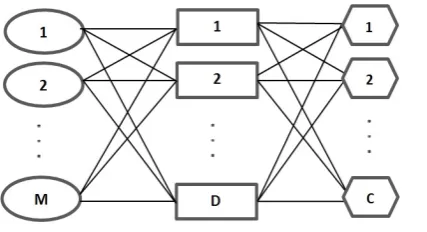
Supply chain network studied in this paper is composed of three main entity types: production centers, distribution centers and demand zones. In the mentioned supply chain network, the raw materials are converted to the finished products and later transformed from the suppliers to the end customers. Supply chain network design consists of the several important strategic decisions in supply chain management, which has an important effect on the overall environmental and economic performance of the supply chain. The main decisions in the supply chain network design are determining locations of network facilities, numbers and capacities of them and the aggregate material flow between facilities. The nature and complexity of today’s supply chains network make them vulnerable to various risks. The structure of the studied supply chain network is graphically depicted in figure 1. The proposed supply chain network is designed under partial and complete facility disruptions. It is assumed that disruptions may be occurred in production and facility centers. To cope with facility disruption, a novel objective function is proposed which minimizes the recovery time of disrupted facilities so that they return to a normal situation from disruption in the shortest possible time. The proposed model considers the following assumptions and limitations:

 The model is single-product and single-period.

 Customer locations and its demands are known and fixed.

 The potential locations of network facilities including manufacturing and distribution centers are known.  The number of potential opened facilities and their capacities are both not restricted and not predetermined.  Supply of production centers and capacity of distribution centers are restricted. Furthermore, all production

centers can send the final product to each distribution center and there isn’t any restriction.  All demand of customers completely must be satisfied.

 Transportation costs between network facilities are known.  Production centers and distribution centers may face disruptions.  Disruption rate can be complete or partial.

 Some factors such as, wage of staff, the price of energy and materials are different, so costs of recovery and outsourcing are not same in all candidate locations.

Fig. 1: Proposed Supply chain network

3.2

Sets, parameters and decision variables

Sets:

(i =1, 2, 3,…, m ) index for production centers

:

i

(j =1, 2, 3,…, d ) j : index for distribution centers

(k =1, 2, 3,…,

c

)

index for demand zones

:

k

Parameters:

𝑭𝑭𝑭𝑭 : Fixed cost of opening of manufacturing facility i

𝑭𝑭𝑭𝑭 ∶ Fixed cost of opening of manufacturing facility j

𝐲𝐲𝐢𝐢𝐢𝐢: Unit transportation cost from ito jper product

𝐲𝐲𝐢𝐢𝐣𝐣: Unit transportation cost from node node j to k per product

𝒔𝒔𝑭𝑭∶ Max supply of manufacturer i

𝒛𝒛𝑭𝑭∶ Capacity of distribution center j

𝐃𝐃𝐣𝐣: Demand in node k

𝒂𝒂𝑭𝑭∶ Percentage of disruption in facility i

𝒂𝒂𝑭𝑭∶ Percentage of disruption in facility j

𝐑𝐑𝐢𝐢: Max protection resource when facility i faces disruption

𝐑𝐑𝐢𝐢: Max protection resource when facility j faces disruption

𝑻𝑻𝑻𝑻𝑭𝑭∶ Total protection budget for production centers in disruption condition

𝑻𝑻𝑻𝑻𝑱𝑱∶ Total protection budget for distribution centers in disruption condition

𝒎𝒎𝑭𝑭∶ Proportion of consumer resource to recovery time in facility i

𝒎𝒎𝑭𝑭∶ Proportion of consumer resource to recovery time in facility j

𝒘𝒘𝑭𝑭∶ Outsourcing cost per time unit in facility i

𝒘𝒘𝑭𝑭∶ Outsourcing cost per time unit in facility j

Decision variables:

𝒒𝒒𝑭𝑭𝑭𝑭 ∶Amount of product flow from node i to j

𝒒𝒒𝑭𝑭𝒋𝒋∶Amount of product flow from node j to k

𝑿𝑿𝑭𝑭 ∶ Is binary, if facility i be open is one, otherwise is 0

𝑿𝑿𝑭𝑭 ∶ Is binary, if facility j be open is one, otherwise is 0

𝒕𝒕𝑭𝑭 : Recovery time for disrupted facility i

𝒕𝒕𝑭𝑭 : Recovery time for disrupted facility j

𝒓𝒓𝒓𝒓𝑭𝑭 ∶ Recovery budget invested for facility i

𝒓𝒓𝒓𝒓𝑭𝑭 ∶Rrecovery budget invested for facility j

𝒐𝒐𝒔𝒔𝒓𝒓𝑭𝑭∶Outsourcing budget invested for facility i

3.3

Model formulation

In this section, a supply chain network is designed under facility disruptions. It is assumed that disruptions are occurred at production and facility centers. To deal with facility disruption, a novel objective function is proposed which minimizes the recovery time of disrupted facilities so that they return to a normal situation from disruption in the shortest possible time. According to the aforementioned definitions and explanations, the proposed bi-objective model for reliable supply chain network design with facility disruption can be written as follows:

minimize � 𝐹𝐹𝐹𝐹 𝑋𝑋𝐹𝐹

𝑚𝑚 𝑖𝑖=1 +� 𝐹𝐹𝐹𝐹 𝑋𝑋𝐹𝐹 𝑑𝑑 𝑗𝑗=1 +� � 𝑞𝑞𝑖𝑖𝑗𝑗 𝑑𝑑 𝑗𝑗=1 𝑚𝑚 𝑖𝑖=1

yij+� �qjk 𝑐𝑐

𝑘𝑘=1 𝑑𝑑

𝑗𝑗=1

𝑦𝑦𝑗𝑗𝑘𝑘+�( 𝑟𝑟𝑟𝑟i 𝑚𝑚

𝑖𝑖=1

+𝑜𝑜𝑜𝑜𝑟𝑟𝑖𝑖) +�( 𝑟𝑟𝑟𝑟j 𝑑𝑑

𝑗𝑗=1

+𝑜𝑜𝑜𝑜𝑟𝑟𝑗𝑗) (1)

� 𝑞𝑞𝑖𝑖𝑗𝑗 𝑑𝑑

𝑗𝑗=1

≤ 𝑜𝑜𝑖𝑖𝑋𝑋𝑖𝑖(1− 𝑎𝑎𝑖𝑖) 𝐹𝐹= 1,2, … ,𝑚𝑚 (2)

� 𝑞𝑞𝑖𝑖𝑗𝑗 𝑚𝑚 𝑖𝑖=1 − � 𝑞𝑞𝑗𝑗𝑘𝑘 𝑐𝑐 𝑘𝑘=1

= 0 𝐹𝐹= 1,2, … , d (3)

� 𝑞𝑞𝑗𝑗𝑘𝑘 𝑑𝑑

𝑗𝑗=1

=𝐷𝐷𝑘𝑘 𝑘𝑘= 1,2, … , c (4)

� 𝑞𝑞𝑖𝑖𝑗𝑗≤ 𝑚𝑚

𝑖𝑖=1

𝑧𝑧𝑗𝑗𝑋𝑋𝑗𝑗�1− 𝑎𝑎𝑗𝑗� 𝐹𝐹= 1,2, … , d (5)

minimize � 𝑡𝑡𝑖𝑖 𝑚𝑚

𝑖𝑖=1

+�tj 𝑑𝑑

𝑗𝑗=1

(6)

𝑟𝑟𝑟𝑟𝑖𝑖=𝑅𝑅𝑖𝑖𝑎𝑎𝑖𝑖𝑋𝑋𝑖𝑖 𝐹𝐹= 1,2, … ,𝑚𝑚 (7)

𝑟𝑟𝑟𝑟𝑗𝑗=𝑅𝑅𝑗𝑗𝑎𝑎𝑗𝑗𝑋𝑋𝑗𝑗 𝐹𝐹= 1,2, … , d (8)

𝑡𝑡𝑖𝑖= (1/𝑚𝑚𝑖𝑖)𝑟𝑟𝑟𝑟𝑖𝑖𝑋𝑋𝑖𝑖 𝐹𝐹= 1,2, … ,𝑚𝑚 (9)

𝑡𝑡𝑗𝑗=�1/𝑚𝑚𝑗𝑗�𝑟𝑟𝑟𝑟𝑗𝑗𝑋𝑋𝑗𝑗 𝐹𝐹= 1,2, … , d (10)

𝑜𝑜𝑜𝑜𝑟𝑟𝑖𝑖= 𝑡𝑡𝑖𝑖𝑤𝑤𝑖𝑖 𝐹𝐹= 1,2, … ,𝑚𝑚 (11)

𝑜𝑜𝑜𝑜𝑟𝑟𝑗𝑗= 𝑡𝑡𝑗𝑗𝑤𝑤𝑗𝑗 𝐹𝐹= 1,2, … , d (12)

� ( 𝑟𝑟𝑟𝑟𝑖𝑖+𝑜𝑜𝑜𝑜𝑟𝑟𝑖𝑖 ) 𝑋𝑋𝑖𝑖≤ 𝑚𝑚

𝑖𝑖=1

𝑇𝑇𝑇𝑇𝑖𝑖 𝐹𝐹= 1,2, … ,𝑚𝑚 (13)

�( 𝑟𝑟𝑟𝑟𝑗𝑗+𝑜𝑜𝑜𝑜𝑟𝑟𝑗𝑗 ) 𝑋𝑋𝑗𝑗≤ 𝑑𝑑

𝑗𝑗=1

𝑇𝑇𝑇𝑇𝑗𝑗 𝐹𝐹= 1,2, … ,𝑑𝑑 (14)

𝑞𝑞𝑖𝑖𝑗𝑗,𝑞𝑞𝑗𝑗𝑘𝑘,𝑟𝑟𝑟𝑟𝑖𝑖 ,𝑟𝑟𝑟𝑟𝑗𝑗,𝑜𝑜𝑜𝑜𝑟𝑟𝑖𝑖,𝑜𝑜𝑜𝑜𝑟𝑟𝑗𝑗,𝑡𝑡𝑖𝑖 ,𝑡𝑡𝑗𝑗 ≥0 ∀ 𝐹𝐹,𝐹𝐹 (15)

𝑋𝑋𝑖𝑖 ,𝑋𝑋𝑗𝑗 ∈{0,1} ∀ 𝐹𝐹,𝐹𝐹 (16)

The objective function (1) minimizes the nominal costs, which include fixed location costs, transportation costs and protection costs after disruptions. The fifth term in the objective function (1) expresses the recovery and outsourcing budgets invested in production facilities when they are faced with disruptions. The last term in the objective function (1) expresses the recovery and outsourcing budgets invested for distribution facilities when they are faced with disruptions. Constraint (2) ensures that the total flow through a production facility does not exceed its capacity, when it is opened. Constraint (3) states that all products shipped from production facilities to a distribution facility must be transported from that distribution facility to customer zones. Constraint (4) ensures that all demand of the customer must be satisfied. Constraint (5) restricts the capacity of distribution facilities.

4.

Solving approach

4.1

ε

-constraint method

Multi-objective optimization programming models simultaneously manipulate several objective functions and are efficient tools to find efficient solutions. An efficient solution has the property, which it is impossible to improve any objective values without sacrificing on at least one other objective [40]. In this paper, the ε-constraint method introduced by Haimes et al. [41] is utilized to provide a set of Pareto-optimal SC configuration. In the ε–constraint, one objective function is optimized while other objectives are considered as constraints with allowable bounds. Then, to generate different Pareto-optimal solutions, the bounds are consecutively modified. The ε–constraint method is formulated as follows:

Min f₁(x)

Subject to:

f

(

x

)

≤

ε

,

f

(

x

)

≤

ε

,...,

f

(

x

)

≤

ε

,

x

∈

S

According to model (17), a set of Pareto-optimal solutions can be obtained by changing values of

ε

ε

ε

4.2

NSGA-II Algorithm

NSGA-II is a popular multi-objective evolutionary algorithm (MOEA), which has three special characteristics, including fast non-dominated sorting approach, fast crowded distance estimation procedure and simple crowded comparison operator [42]. NSGA-II is population-based search MOEA that can generate a set of Pareto Optimal solutions involving two or more conflicting objectives. One of these MOEAs that was frequently used in many optimization problems as the best Technique to generate Pareto frontiers is the non-dominated sorting genetic algorithm-II (NSGA-II) proposed by Deb et al. [42]. Deb et al. [42] designed several test problems using NSGA-II optimization technique. The authors compared NSGA-II with other MOEAs and claimed that this technique outperformed PAES (Pareto-archived evolution strategy) and SPEA (strength Pareto evolutionary algorithm) in terms of finding a diverse set of solutions [43-44]. The chromosome encoding in NSGA-II algorithm is described below.

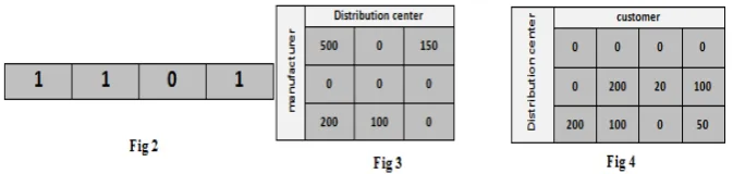
Chromosome encoding

Encoding is used to translate a genetic solution of the problem into a chromosome string suitable to the application of genetic operators. For our problem, the chromosome contains four sections. First and second sections belong to close or open of manufacturers and distributed facility. (Fig 2) Third and fourth section present the transportation matrix from manufacturers to distribution centers and from distribution centers to customers (Fig 2, 3, 4).

Fig 2 present a manufacturer or distribution centers chromosome with four candidate facility, that facility 3 is close.

NSGA II Algorithm steps

Initialization

In this step of the algorithm we generate random chromosome to the number of primary generation size. Then eliminate infeasible chromosomes. Hence resume this generation, up to we have feasible chromosome to the number of primary generation size. Then, we evaluate chromosome according to their objective functions and use Fast non-dominated sorting method and crowding distance for sorting of chromosomes.

Selection strategy

crowding distance, second parent is selected with the same method. Hence we have two parent chromosomes for generating new offspring.

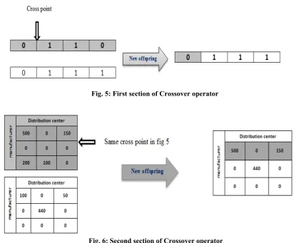
Crossover Operator

After selection of two chromosomes with tournament method as parents, we use the crossover operator for generating better offspring by combining the selected parents directly with probability pc. In crossover operator, first we select one chromosome from one of manufacturers or distribution centers with 1/2 probability, then one point of this chromosome is selected randomly, and then two parts of this chromosome are displaced. Assume manufacturer is selected. (See fig 5).

Fig. 5: First section of Crossover operator

Fig. 6: Second section of Crossover operator

After performing above operations, we first consider feasibility of offspring generation, if new offspring is feasible, it is compared to all answers of last front, if it is better, the new generated offspring is transferred to the next generation.

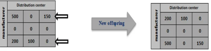
Mutation Operator

In mutation operator each offspring is assigned a small probability of mutation, so that the solutions are more diversified. With probability pm, select an individual from the population and swap two random genes. For mutation operator, we first select one of the manufacturers or distribution centers with probability ½ and select a chromosome randomly.

Fig. 8: Second section of mutation operator

After performing above operations, we first consider feasibility of offspring generation, if new offspring is feasible, it is compared to all answers of last front, if it is better, the new generated offspring is transferred to the next generation.

Termination criteria

Algorithm terminates when maximum generation is achieved.

Archive Operator

After crossover and mutation operators, we archive all solutions in first front. Hence, after completion of the maximum generation (termination conditions) we have an archive from all solutions on first front in any generation. Finally, we sort all solutions in the archive, and solutions in first front are the final solution.

5.

Computational results

The studied problem is solved on a Pentium dual-core 2.20 GHz computer with 4.00 GB RAM in order to generate a different Pareto optimal solution. First for evaluation of NSGA II Algorithm we generated 8 random data sets of different problems with small sizes and the results compared with ε-constraint method. (See table 1)

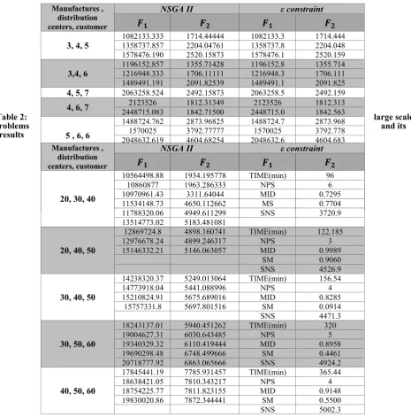
For large scale problem, we generated 5 problems with random data. For design of experimental problems, we fixed cost for opening of manufacturers facility is drawn uniformly (200000, 550000), and for distribution centers is (50000, 100000), unit transportation costs are uniformly (200, 1000), max supply of manufacturer and Capacity of distribution centers are uniformly (500, 2000), (1500, 4000) respectively, demand of customers is uniformly (200, 450), probability disruption for manufacturers and distribution centers are uniformly (0, 1), max protection resource for manufacturers and distribution centers are uniformly (2000, 7000) ,(1000, 3000) , proportion of consumer resource to recovery time for manufacturers and distribution centers are uniformly (5,15) ,(2, 8) , Outsourcing cost for per time unit for manufacturers and distribution centers are uniformly (20,40) ,(10, 25).

For small scale of this model, we used ε constraint method and solve the problem in GAMS software and for large scale problems, we coded problem with NSGAII in MATLAB. For validation of NSGAII algorithm, we solved small scale problem with this algorithm and for the future comparisons of NSGA II. As Table 1 shows the results of NSGA II and ε constraint method are similar for small scale problems. Therefore, it is recommended that ε constraint method should be used as an exact method to obtain Pareto optimal solutions.

Table 1: Small scale problems and compare results of NSGA II and ε constraint method

Table 2: large scale

problems and its

results

Also best non-dominated solutions for large scale problems indicated in fig 9 – 13.

Manufactures , distribution centers, customer

NSGA II ε constraint

𝑭𝑭

𝑭𝑭

𝑭𝑭

𝑭𝑭

3, 4, 5 1082133.3331358737.857 1714.444442204.04761 1082133.31358737.8 1714.4442204.048

1578476.190 2520.15873 1578476.1 2520.159

3,4, 6 1196152.8571216948.333 1355.714281706.11111 1196152.81216948.3 1355.7141706.111

1489491.191 2091.82539 1489491.1 2091.825

4, 5, 7 2063258.524 2492.15873 2063258.5 2492.159

4, 6, 7 _2448715.0832123526 1812.31349_{1842.71500 2448715.0}2123526 1812.313_1842.563

5 , 6, 6

1488724.762 2873.96825 1488724.7 2873.968

1570025 3792.77777 1570025 3792.778

2048632.619 4604.68254 2048632.6 4604.683

2365701.191 5077.65873 2365701.1 5077.658

5,7, 8 2333250.952 3846.62698 2333250.9 3846.623

6, 8,9 2403259.2862875385.868 4875.571424917.4329 2403259.22875385.8 4875.5674910.29

3180294.558 5162.31385 3180294.5 5163.147

6, 8,10 _3404610.5582705498.63 4923.62337_5162.31385 2705498.6_3404610.5 4923.214_5162.314

Manufactures , distribution centers, customer

NSGA II ε constraint

𝑭𝑭

𝑭𝑭

𝑭𝑭

𝑭𝑭

20, 30, 40

10564498.88 1934.195778 TIME(min) 96

10860877 1963.286333 NPS 6

10970961.43 3311.64044 MID 0.7295

11534148.73 4650.112662 MS 0.7704

11788320.06 4949.611299 SNS 3720.9

13514773.02 5183.481081

20, 40, 50

12869724.8 4898.160741 TIME(min) 122.185

12976678.24 4899.246317 NPS 3

15146332.21 5146.063057 MID 0.9989

SM 0.9060

SNS 4526.9

30, 40, 50

14238320.37 5249.013064 TIME(min) 156.54

14773918.04 5441.088996 NPS 4

15210824.91 5675.689016 MID 0.8285

15757331.8 5697.801516 SM 0.0914

SNS 4471.3

30, 50, 60

18243137.01 5940.451262 TIME(min) 320

19004627.31 6030.643485 NPS 5

19340329.32 6110.419444 MID 0.8958

19690298.48 6748.499666 SM 0.4461

20718777.92 6863.065666 SNS 4924.2

40, 50, 60

17845441.19 7785.931457 TIME(min) 365.44

18638421.05 7810.343217 NPS 4

18754225.77 7811.823155 MID 0.9148

19830020.86 7872.344441 SM 0.5500

6.

Conclusion and suggestions for further research

solved small scale problem with this algorithm and for the future comparisons of NSGA II, we calculated some criteria like NPS, MID, SNS and MS. Results are demonstrated in computational results section.

There are some potential directions for future works. Our proposed model is a single period and model will be more real and some parameters will have different behavior in multi period model. Another subject that can be considered in future research is some parameters have stochastic nature and present a robust model for SCND. Also, we can integrate the reverse logistic follow into the forward flow and study the influence of recovery time and protection resources in a closed loop supply chain network.

Acknowledgement

This work has been financially supported by the research deputy of Shahrekord University. The grant number was 97GRN1M1759.

References

[1] Kleindorfer, P. R. and G. H. Saad (2005). "Managing Disruption Risks in Supply Chains." Production and Operations Management 14(1): 53-68.

[2] Hishamuddin, H., R. A. Sarker and D. Essam (2013). "A recovery model for a two-echelon serial supply chain with consideration of transportation disruption." Computers & Industrial Engineering 64(2): 552-561.

[3] Chopra, S. and M. S. Sodhi (2004). "Managing risk to avoid supply chain breakdown." Sloan Management Review 46(1): 53–62.

[4] Tang, O. and S. Nurmaya Musa (2011). "Identifying risk issues and research advancements in supply chain risk management." International Journal of Production Economics 133(1): 25-34.

[5] Hall, P. V. (2004). "“We’d Have to Sink the Ships”: Impact Studies and the 2002 West Coast Port Lockout." Economic Development Quarterly 18(4): 354-367.

[6] Sheffi, Y. and J. Rice (2005). " A supply chain view of the resilient enterprise." MIT Sloan Management Review 47(1): 41–48.

[7] Davarzani, H., S. H. Zegordi and A. Norrman (2011). "Contingent management of supply chain disruption: Effects of dual or triple sourcing." Scientia Iranica 18(6): 1517-1528.

[8] Knemeyer, A. M., W. Zinn and C. Eroglu (2009). "Proactive planning for catastrophic events in supply chains." Journal of Operations Management 27(2): 141-153.

[9] Wagner, S. M. and C. Bode (2008). "An empirical examination of supply chain performance along several dimensions of risk." Journal of Business Logistics 29(1): 307-325.

[10] Klibi, W. and A. Martel (2012). "Scenario-based Supply Chain Network risk modeling." European Journal of Operational Research 223(3): 644-658.

[11] Franca, R. B., E. C. Jones, C. N. Richards and J. P. Carlson (2010). "Multi-objective stochastic supply chain modeling to evaluate tradeoffs between profit and quality." International Journal of Production Economics 127(2): 292-299.

[12] Schmitt, A. J., L. V. Snyder and Z.-J. M. Shen (2010). "Inventory systems with stochastic demand and supply: Properties and approximations." European Journal of Operational Research 206(2): 313-328.

[13] Tomlin, B. (2006). "On the Value of Mitigation and Contingency Strategies for Managing Supply Chain Disruption Risks." Management Science 52(5): 639-657.

[14] Azad, N., H. Davoudpour, G. K. D. Saharidis and M. Shiripour (2014). "A new model to mitigating random disruption risks of facility and transportation in supply chain network design." The International Journal of Advanced Manufacturing Technology 70(9): 1757-1774.

[15] Friesz, T. L., I. Lee and C.-C. Lin (2011). "Competition and disruption in a dynamic urban supply chain." Transportation Research Part B: Methodological 45(8): 1212-1231.

[16] Losada, C., M. P. Scaparra and J. R. O’Hanley (2012). "Optimizing system resilience: A facility protection model with recovery time." European Journal of Operational Research 217(3): 519-530.

[17] Melo, M. T., S. Nickel and F. Saldanha-da-Gama (2009). "Facility location and supply chain management – A review." European Journal of Operational Research 196(2): 401-412.

[18] Tang, C. S. (2006). "Robust strategies for mitigating supply chain disruptions." International Journal of Logistics Research and Applications 9(1): 33-45.

[19] Drezner, Z. (1987). "Heuristic Solution Methods for Two Location Problems with Unreliable Facilities." Journal of the Operational Research Society 38(6): 509-514.

[20] Snyder, L. V. and M. S. Daskin (2005). "Reliability Models for Facility Location: The Expected Failure Cost Case." Transportation Science 39(3): 400-416.

[22] Li, X. and Y. Ouyang (2010). "A continuum approximation approach to reliable facility location design under correlated probabilistic disruptions." Transportation Research Part B: Methodological 44(4): 535-548.

[23] Lim, M., M. S. Daskin, A. Bassamboo and S. Chopra (2010). "A facility reliability problem: Formulation, properties, and algorithm." Naval Research Logistics (NRL) 57(1): 58-70.

[24] Snyder, L. V. (2006). "Facility location under uncertainty: a review." IIE Transactions 38(7): 547-564.

[25] Shao, X.-F. (2012). "Demand-side reactive strategies for supply disruptions in a multiple-product system." International Journal of Production Economics 136(1): 241-252.

[26] Hatefi, S. M. and F. Jolai (2014). "Robust and reliable forward–reverse logistics network design under demand uncertainty and facility disruptions." Applied Mathematical Modelling 38(9–10): 2630-2647.

[27] Hatefi, S. M. and F. Jolai (2015). "Reliable forward-reverse logistics network design under partial and complete facility disruptions." International Journal of Logistics Systems and Management 20(3): 370-394.

[28] Torabi, S., J. Namdar, S. Hatefi and F. Jolai (2016). "An enhanced possibilistic programming approach for reliable closed-loop supply chain network design." International Journal of Production Research 54(5): 1358-1387.

[29] Hatefi, S. M., F. Jolai, S. A. Torabi and R. Tavakkoli-Moghaddam (2015). "A credibility-constrained programming for reliable forward–reverse logistics network design under uncertainty and facility disruptions." International Journal of Computer Integrated Manufacturing 28(6): 664-678.

[30] Hatefi, S. M., F. Jolai, S. A. Torabi and R. Tavakkoli-Moghaddam (2015). "Reliable design of an integrated forward-revere logistics network under uncertainty and facility disruptions: A fuzzy possibilistic programing model." KSCE Journal of Civil Engineering 19(4): 1117-1128.

[31] Hatefi, S. M., F. Jolai, S. A. Torabi and R. Tavakkoli-Moghaddam (2016). "Integrated Forward-reverse Logistics Network Design under Uncertainty and Reliability Consideration." Scientia Iranica. Transaction E, Industrial Engineering 23(2): 721-735.

[32] Azad, N., G. K. D. Saharidis, H. Davoudpour, H. Malekly and S. A. Yektamaram (2013). "Strategies for protecting supply chain networks against facility and transportation disruptions: an improved Benders decomposition approach." Annals of Operations Research 210(1): 125-163.

[33] Jabbarzadeh, A., B. Fahimnia, J. B. Sheu and H. S. Moghadam (2016). "Designing a supply chain resilient to major disruptions and supply/demand interruptions." Transportation Research Part B: Methodological 94: 121-149.

[34] Jabbarzadeh, A., B. Fahimnia, et al. (2018). "Resilient and sustainable supply chain design: sustainability analysis under disruption risks." International Journal of Production Research 56(17): 5945-5968.

[35] Namdar, J., X. Li, et al. (2018). "Supply chain resilience for single and multiple sourcing in the presence of disruption risks." International Journal of Production Research 56(6): 2339-2360.

[36] Paul, S. K., R. Sarker, et al. (2018). "A reactive mitigation approach for managing supply disruption in a three-tier supply chain." Journal of Intelligent Manufacturing 29(7): 1581-1597.

[37] Ghavamifar, A., A. Makui, et al. (2018). "Designing a resilient competitive supply chain network under disruption risks: A real-world application." Transportation Research Part E: Logistics and Transportation Review 115: 87-109.

[38] Diabat, A., A. Jabbarzadeh, et al. (2019). "A perishable product supply chain network design problem with reliability and disruption considerations." International Journal of Production Economics 212: 125-138.

[39] Sahebjamnia, N., S. A. Torabi and S. A. Mansouri (2015). "Integrated business continuity and disaster recovery planning: Towards organizational resilience." European Journal of Operational Research 242(1): 261-273.

[40] Amin, S. H. and G. Zhang (2013). "A multi-objective facility location model for closed-loop supply chain network under uncertain demand and return." Applied Mathematical Modelling 37(6): 4165-4176.

[41] Haimes, Y. Y., L. S. Lasdon and D. A. Wismer (1971). "On a Bicriterion Formulation of the Problems of Integrated System Identification and System Optimization." IEEE Transactions on Systems, Man, and Cybernetics SMC-1(3): 296-297.

[42] Deb, K., A. Pratap, S. Agarwal and T. Meyarivan (2002). "A fast and elitist multi objective genetic algorithm: NSGA-II." IEEE Transactions on Evolutionary Computation 6(2): 182-197.

[43] Kodali, S. P., R. Kudikala and D. Kalyanmoy (2008). Multi-Objective Optimization of Surface Grinding Process Using NSGA II. 2008 First International Conference on Emerging Trends in Engineering and Technology. [44] Chen, J. (2009). Multi-Objective Optimization of Cutting Parameters with Improved NSGA-II. 2009 International

Conference on Management and Service Science.