The Effects of Different SDE Calculus on Dynamics of Nano-Aerosols Motion in Two Phase Flow Systems

(1)

35

The Effects of Different SDE Calculus on Dynamics of

Nano-Aerosols Motion in Two Phase Flow Systems

F. Hosseinibalam, S. Hassanzadeh and O. Ghaffarpasand

*

Physics Department, Faculty of Sciences, University of Isfahan, Isfahan, I.R. Iran

(*) Corresponding author: [email protected]

(Received: 14 Oct. 2010 and Accepted: 1 2 Mar. 2011)

Abstract:

Langevin equation for a nano-particle suspended in a laminar fluid flow was analytically studied. The Brownian motion generated from molecular bombardment was taken as a Wiener stochastic process and approximated by a Gaussian white noise. Euler-Maruyama method was used to solve the Langevin equation numerically. The accuracy of Brownian simulation was checked by performing a series of simulations. Particles’ trajectories for an ensemble of 1000 particles were calculated and compiled by Lagrangian approach. Numerical simulation in cartesian coordinate were validated by exact solution of Einstein and good agreement was observed. Moreover, strong convergence of proposed method has been considered. The approximated scheme has strong order of convergence, 1.5. Langevin equations in cylindrical coordinate were also considered as stochastic differential equations (SDE) and in different SDE calculus were solved numerically by validated numerical method. A novel approach to simulating the Brownian motion as the Gaussian white noise is presented in cylindrical coordinates. Obtained results for different SDEs calculus were compared and suggested that there are no considerable differences between Ito and Stratonovich approaches in two phase flow systems.

Keywords: Stochastic Differential Equation (SDE), Nano-Aerosol (NA), Laminar Fluid, Stratonovich, Ito.

1. INTRODUCTION

Studying the dynamics of aerosols motion has attracted attentions in the past two decades. An aerosol is defined as a collection of solid or liquid particles suspended in a gas. Aerosols are at least two-phase systems, consisting of particles and gas in which they are suspended [1-3].

They are also one of the major air pollutants and recent studies of the biological effects of nano-aerosols (NAs) show signs that some manufactured NAs display unexpected toxicity to living organisms. Some of these particles can become potentially harmful and even cause deleterious health effects [4, 5].

Analyzing the diffusion of small aerosols has considerable effects on controlling and measuring

the aerosol concentration in different area [5-7] because particle diffusion plays a major role in aerosol transportation mechanisms [5]. One of the common types of diffusion is Brownian diffusion which has important role in transfer mechanisms of ultrafine particles.

(2)

36

scientists [10, 11]. Yet, to our knowledge, nobody has considered the Brownian motion in cylindrical coordinate and/or different SDE calculus (Ito and Stratonovich). The difference between Ito and Stratonovich calculus is evident from the different choices of the intermediate points in describing the stochastic integrals (see appendix A). Ito definition is recommended by mathematicians, but the physicists prefer the Stratonovich advantages. In particular, physicists argued that the physical processes are actually smooth on extremely short time scales, order of molecular collision times,

and hence in physical phenomena the Stratonovich definition is recommended.

In light of the above discussion, the main goal of this study concerns the fundamental understanding of how Brownian motion and numerical simulations can be applied for ultrafine aerosols within the frameworks of different SDE calculus and/or in cylindrical coordinate.

This paper is organized as follow: in section 2, dynamics of a nano aerosol motion in 1D cartesian coordinates was described and an approximate term for Brownian motion was presented. In section

11

Tables

P(P Oper Pres 30

ࢊࡼ(n

Particle D 3 1 3 10

Figures

Figu T Pa) rating sure 00 T nm) Diameter 3 0 0 00

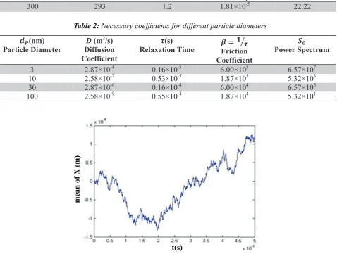
ure 1:Mean d

Table 1: Oper

T(K) Temperatu

293

Table 2:Nece

ࡰ (m2_/s) Diffusion Coefficien 2.87×10-4 2.58×10-7 2.87×10-6 2.58×10-9 displacement rating conditi ure ࣋ essary coeffici ) n nt Rela 4 ₀ 7 ₀ 6 ₀ 9 ₀

t of ensembles

ions and carr

࣋ (Kg/m3₎

1.2

ients for diffe

࣎(s) axation Time 0.16×10-5 0.53×10-5 0.16×10-4 0.55×10-4

s of ultrafine

rier gas (air) p

ࣆ (P Dyn Visc

1.81

erent particle

e ࢼ ൌ_Fric Coeff

6.00 1.87 6.00 1.87

aerosols (݀௉

properties Pa.s) namic cosity O ×10-5 diameters ൌ ૚ ࣎ൗ ction ficient 0×105 7×105 0×104 7×104 =10nm) susp

ࣅ (ࣆm) Mean Free Pa Operating Pre 22.22 ࡿ૙ Power Spect 6.57×10 5.32×10 6.57×10 5.32×10

pended in air.

ath at essure trum 7 3 3 1

Tables

P(P Oper Pres 30

ࢊࡼ(n Particle D 3 1 3 10

Figures

ure 1:Mean d

Table 1: Oper

293

Table 2:Nece

ࡰ (m2_/s) Diffusion Coefficien 2.87×10-4 2.58×10-7 2.87×10-6 2.58×10-9 displacement rating conditi ure ࣋ essary coeffici ) n nt Rela 4 ₀ 7 ₀ 6 ₀ 9 ₀

t of ensembles

ions and carr

࣋ (Kg/m3₎

1.2

ients for diffe

࣎(s) axation Time 0.16×10-5 0.53×10-5 0.16×10-4 0.55×10-4

s of ultrafine

rier gas (air) p

ࣆ (P Dyn Visc

1.81

erent particle

6.00 1.87 6.00 1.87

aerosols (݀௉

pended in air.

ath at essure trum 7 3 3 1

Ghaffarpasand,

et al.

Table 1: Operating conditions and carrier gas (air) prperties

Table 2: Necessary coefficients for different particle diameters

11

Tables

P(P Oper Pres 30

ࢊࡼ(n Particle D 3 1 3 10

Figures

ure 1:Mean d

Table 1: Oper

293

Table 2:Nece ࡰ (m2_/s) Diffusion Coefficien 2.87×10-4 2.58×10-7 2.87×10-6 2.58×10-9 displacement rating conditi ure ࣋ essary coeffici ) n nt Rela 4 ₀ 7 ₀ 6 ₀ 9 ₀

t of ensembles

ions and carr ࣋ (Kg/m3₎

1.2

ients for diffe ࣎(s) axation Time 0.16×10-5 0.53×10-5 0.16×10-4 0.55×10-4

s of ultrafine

rier gas (air) p ࣆ (P Dyn Visc

1.81

erent particle

6.00 1.87 6.00 1.87

aerosols (݀௉

pended in air.

ath at essure trum 7 3 3 1 t(s)

(3)

37

3 equation of motion was numerically solved by

the approximated term. Numerical method was validated by comparing the elaborated results with exact solution of equation of motion and its order of convergence evaluated. In section 4 equation of motion of a nano particle in cylindrical coordinates

was analytically investigated and the effects of different SDE calculus was studied. In section 5 equation of motion in cylindrical coordinates was numerically solved by validated numerical method. Finally, we compare the results and conclusion will be presented.

(4)

2. LANGEVIN EQUATION

The equation of motion of an ultrafine aerosol which suspended in a laminar gas flow called Langevin which is given below for a dilute gas-particle flow [12]:

(1)

where V_P is the particle velocity vector, F_D is the drag force per unit mass, F_Bis a fluctuating

(5)

39

that, the dominant forces in motion of an ultrafine

aerosol are Drag and Brownian forces which will be further described.

2.1. Drag force

The expression for the modified Stokes drag force per unit mass is given by [2]:

(2)

Here V_f is the velocity vector of carrier fluids, is the drag coefficient, where d_p is particle diameter, m_p is mass of the particle, µ is the coefficient of dynamic viscosity and C_C is the Cunningham slip correction factor which is:

(3)

where P is the absolute pressure in kPa and d_p is the particle diameter in µm. As it was mentioned before, particle concentration was assumed too low and, so, the effects of particle motion on the carrier fluids can be ignored. On the other hand, suspended particles in laminar fluid flow in parallel layers. As there is no any solid boundary, the velocity vector of carrier fluid can be considered as a constant value and, in this case, it can be neglected in numerical integrations and analytical investigations of Langevin equation.

2.2. Brownian Motion

It is well known that the Brownian motion of nano-aerosols is due to random impact of gas molecules. If x(t) denotes the position of a particle at time t, then the displacement x(t)-x(0) is the effect of the purely random bombardment by the molecules of fluids. Figure 1 shows the tracks for ensembles of ultrafine aerosols which were suspended in ambient air and affected by bombardment of air molecules. Wiener (1931) considered the position of an ultrafine particle which suspended in a dilute carrier gas as a stochastic process. He found that the fluctuating

part of equation of motion, F_B(t), have following properties [13]:

1.

Independence of increments: There will be correlation between the values of F_B(t) at different times t₁ and t₂ only when is very small:

(4)

where is a function and has a very sharp maximum at z=0.

International Journal of Nanoscience and Nanotechnology

14

Figgure 6: Stronng convergencce of presenteed model in (a

(a) Ito and (b)

) Stratonovicch definition.

14

Figgure 6: Stronng convergencce of presenteed model in (a

(a) Ito and (b)

(6)

2.

Normal increments: has normal distribution with zero mean and variance t₁-t₂:

(5)

3.

Continuity of paths: is

continuous function of t.

Now we can write the Langevin equation (1) as

follow:

(6)

where b is drag coefficient which mentioned in section 2.1. By integrating the above differential equation we can get:

(7)

15

Figuree 7:Sum of me

cylindricalean square vecoordinateselocity compo(Stratonovich

(a)

(b)

(c)

onents in (a) c

h definition) aand (c) 1D cacylindrical co

oordinates (Ito

(7)

41

By taking the mean over an ensemble of particles,

and using (5) we get:

(8)

The mean velocity goes down exponentially due to the friction coefficient. Calculating the mean by squaring the equation (7), gives:

(9)

The new variables

are introduced, then by using (4) the above integral is:

(10)

where τ is defined as:

(11)

We know from the theorem of equipartition of energy and kinetic theory of gases, the following condition:

(12)

where k_B is the Boltzman constant and T is the temperature. By using the equations (9), (10), and (12) the value of t is obtained as follow:

(13)

A definition for f(z) can be derived by using equations (11), (12), and help of dirac delta function property as follows:

(14)

It was known that autocorrelation of a random process describes the correlation between values of the process at different time. The Fourier transform of autocorrelation was also defined as power spectrum of random process. A stochastic process is called

white noise when its power spectrum is independent of frequency. The name white noise comes from the fact that its power spectrum is uniformly distributed in frequency, which is a characteristic of white light. The equation (14) proved that the autocorrelation of (power spectrum) of Brownian motion is independent of time (frequency).

From this fact and the second property of the Brownian motion (equation (5)) it proved that the Brownian motion in 1D cartesian coordinate can be approximated by a Gaussian white noise process when its power spectrum is equal to .

3. NUMERICAL VALIDATION

3.1. Exact solution

The famous Einstein relation between the diffusion coefficient and the long time behavior of the mean-square displacements of an ultrafine particle as a function of time is the basis of numerical validation of elaborated term for Brownian motion. Diffusion of aerosol particles is the net transport of these particles in a concentration gradient. This transport is always from a region of higher concentration to a region of lower concentration. The Einstein relation (following equation) is important equation that relates the diffusion coefficient to mean square displacement of an aerosol in each cartesian coordinates.

3.2. Numerical simulation

Under typical operating two phase flow conditions, particle concentration are low enough and because particle-particle interactions are negligible the presence of particles does not affect the carrier gas flow fields. Particle trajectories were obtained by a Lagrangian approach. In order to investigate the effect of Brownian diffusion in Lagrangian calculations, one needs to add the random Brownian force to Newton’s equation of motion along with the deterministic drag term.

(8)

In section 2.2, we mentioned the physical meaning of Brownian effect which approximated by a Gaussian white noise and obtained as equation (14). To construct a computer simulation of the Langevin equation, the delta function of the white noise needs to be replaced by a numerical representation as [15]:

(17)

Thus, the Brownian force per unit mass in 1D

cartesian coordinates within each time step can be written as:

(18)

A is a constant which represents a zero mean Gaussian random numbers with unit variance. Power spectrum, S₀, can be defined as:

(19)

where v is kinematic viscosity coefficient of fluid. There are different numerical methods that can integrate the Langevin equation. Euler-Maruyama and Rung-Kutta are such that familiar methods. Euler- Maruyama Method which is simpler and faster was used to integrate the Langevin equation numerically [14]. Furthermore, it will be shown that this method, in this case, has an acceptable order of convergence in comparison to the other methods. In this method, the equation of motion was numerically integrated by an explicit Euler method. The value of Brownian force which was defined as equation (18) have been changed in each time step by a Gaussian random number generator.

The simulation time steps, ∆t, is assumed to be larger than the time step between successive collisions of the particle with the surrounding fluid molecules (contact time during a collision ~ picoseconds), but much smaller than the time step associated with an appreciable change in the particle displacement due to the friction forces (order of magnitude of inertial relaxation time of particles ~ microseconds). Thus, we are concerned with time steps of the order of momentum relaxation time (β-1_{) or greater [16].} Operating pressure was taken low enough (300Pa) so that particle-particle interactions are negligible. Air in ambient condition was considered as carrier gas. The operating conditions and carrier gas (Air) properties are gathered in Table1. Table 2 shows the relevant coefficients of particles with different size, where the ratio of the particle density to fluid density is 2000.

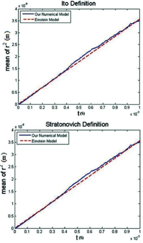
Einstein (1909) obtained the diffusion theory of suspended particles, which described the relation of mean square displacement of particles in 1D cartesian coordinate as a function of time

(9)

43

. As there are no any analytical solutions

for equation of motion in cylindrical coordinate, the presented model was validated by this theory and then used to simulate the motion of particles in cylindrical coordinates.

The ensembles of 1000 particles, which are distributed uniformly in a domain with a dimension of 5mm, were used to compute the mean-square displacement. The ensemble improves the accuracy of the simulation procedure. Different particle diameters (3, 10, 30 and 100 nm) were used to improve the validation procedure. The results were obtained from simulation are shown in figures 2-6. As we can see from figures, the results are in good agreement with the diffusion theory of Einstein. Observed deviations are, may be, due to the fluctuations which were generated by random number generator in each time step.

3.3. Strong convergence of the model

It is known that [17] the exact solution of Langevin

equation in 1D

cartesian coordinate is:

(20) where V_x(0) is initial velocity which is assumed to be zero. This process is called Ornstein-Uhlenbeck process which has different answers in different SDE calculus.

The model is said to have strong convergence equal γ if there exists a constant C such that

(21)

where E|X_n and X(τ)| are the expected value. Strong convergence of numerical methods gives a measure of the path wise closeness at the end of the time interval. In the other word, it’s a measure of agreement between numerical and exact results. Strong approximations involve simulating the solution of SDEs when a good path wise approximation is required.

For evaluating the order of convergence the exact and numerical solutions of considered SDE were investigated at any fixed point (∆t is sufficiently small). On the other hand, the error takes into account at the end point, thus we can write:

(22).

Stochastic integral in equation (20) was solved by the Ito and the Stratonovich definition which represent different stochastic calculus. The Ito and Stratonovich calculus are provided in Appendix A. Thousands of different Brownian paths of ultrafine aerosols (diameter of 10nm) were computed over [0.5×10-6_{] with δt=0.05×10}-5_{. For each path, five} different step sizes: ∆t=2(p-1)_{δt for 0≤p≤1 were} used. For reference, a dashed line of slope 1.5 is added. Converging was tested separately in Ito and Stratonovich definitions.

As we can see from figure 5 the slop of lines are well matched. The results of calculations show that: γ=1.4693 and C=0.4349 for Stratonovich definition and γ=1.5293 and C=0.5258 for Ito definition. Hence our results are consistent with a strong order of convergence equal 1.5.

It was known that [17] the Runge-Kutta method with strong order of convergence equal 1.5 is one of the best accurate methods to investigate the SDEs. As it was observed, Euler-Maruyama method for investigating the motion of nano-particles is an acceptable method both in terms of simplicity and accuracy.

4. LANGEVIN EQUATION IN CYLINDRICAL COORDINATES

Up to now, it was shown that Langevin equation of an ultrafine particle, which suspended in a dilute laminar flow, in 1D cartesian coordinate can be represented by a SDE, from here the motion of particles in 2D cartesian and cylindrical coordinates are considered. In this section equation of motion in cylindrical coordinates and in different SDE calculus (Ito and Stratonovich) were studied analytically. The relations for transforming between coordinates are not similar for different SDE calculus [17].

International Journal of Nanoscience and Nanotechnology

4.1. Ito definition of Langevin equation

7

Ito definition of Langevin Equation

Langevin equation in 2D cartesian coordinates could be represented as:

�_��

� � �� (23)

where �� , �� , and ��

are the particle velocity components. It is clear that the following relations exist between components of displacement and velocity in cartesian and cylindrical coordinates.

� � ��_{� �}�₍₂₄₎

� � ��_��

��; (25)

�_��

� � �� (26)

where �� _�� , and �� _�� are the radial

component and the tangential component of velocity, respectively.

Ito calculus provides a relation for changing the variables, which states that if:

�� (27)

where ��, �� are m-dimensional vectors,

�� is a n-dimensional process and �� is a m × n matrices. Then for every m-dimensional function, ��, with continuous partial derivatives up to order two we can write:

�� _�� ∑��

�∑�� ∑�� ∑��∑�� (28) where ��_��_�.

By using the Ito formula and equations (26):

� ��

��

�� _��

�

(29) We can define:

�_��

� ��_{�� }�� _��

�� (30)

It is shown that (see appendix B) If � is an orthogonal � � � matrix, i.e. �� _{� �}_{, and}_�_is

a d-dimensional standard Gaussian vector, then

�� is also a d-dimensional standard Gaussian vector. As the Brownian motion defined as a Gaussian function, and above � � � matrix is an orthogonal matrix, it can be concluded that Brownian motion in radial and tangential direction can be also considered as a Gaussian white noise and, so, the Ito definition of nano-aerosol motion in cylindrical coordinates are:

� ��

�� _��

� (31)

Stratonovich definition of Langevin Equation It is also possible to write a SDE using Stratonovich approach. There is a specific relation between Ito and Stratonovich definition [17]. If Ito’s equation for multiple variables was written as:

�� (32)

Then, it can be shown that by the following transformation:

�� _�∑ �� (33) �� (34)

The corresponding Stratonovich equation can be generated. By substituting the equation (31) in (33) and (34), Langevin equations in cylindrical coordinates in Stratonovich definition are:

� �� _��

� � �

��

�� _��_��_��

(35)

(10)

44 Ghaffarpasand,

et al.

7

�_��

� � �� (23)

where �� , �� , and �� are the particle velocity components. It is clear that the following relations exist between components of displacement and velocity in cartesian and cylindrical coordinates.

� � ��_{� �}�₍₂₄₎ � � ��_��

��; (25)

�_��

� � �� (26)

where �� _�� , and �� _�� are the radial component and the tangential component of velocity, respectively.

�� (27)

�� _�� ∑��

�∑�� ∑��

∑��∑�� (28)

where ��_�� .

� �� _�� (29) We can define:

�_��

� � ��

� ��_{�� }�� _��

�� (30)

It is shown that (see appendix B) If � is an orthogonal � � � matrix, i.e. �� _{� �}_{, and}_�_is a d-dimensional standard Gaussian vector, then

� ��

��

�� _��

� (31)

�� (32)

�� _�∑ �� (33)

�� (34)

� �� _�� _��_��_�� (35)

�_��

� � �� (23)

where �� , �� , and ��

� � ��_{� �}�₍₂₄₎

� � ��_��

��; (25)

�_��

�� (26)

�� (27)

�� _�� ∑��

�∑�� ∑�� ∑��∑�� (28)

where ��_�� .

� �� _�� (29) We can define:

�_��

� ��_{�� }�� _��

�� (30)

� �� _��

�� _��

� (31)

�� (32)

�_�� _{� �}

��_�∑ �� (33) �_�� _{� �}

�� (34)

� �� _��_��_�� (35) 8

The additional terms (�_��

� and��

�

��) were added in comparison to the Ito definition. These differences will be studied in the next section, when the numerical investigations of equation of motion in different SDE calculus are presented.

Numerical Simulation of the Langevin Equation in Cylindrical Coordinates

Langevin equation in cylindrical coordinates for radial and tangential components of velocity (equations (31) and (35)) was solved by approximate model which was described in section 2. The spherical particles, 10nm in diameter, were assumed to be uniformly distributed in a tube with a diameter of 10mm.The operating conditions are the same as the validation conditions given in tables 1 and 2. As we can see from equation (26), there exists a specific relation between velocity components in the cartesian and cylindrical coordinates as follow:

��

�� (36)

Figure 7 shows the sum of mean of velocity components in different coordinates and different calculus. On the other hand, mean square displacement of radial component is considered in figures 8. Two important results can be found by analyzing these figures. First, it was seen that there is no significant difference between Ito and Stratonovich definition, in the other point, both definitions lead to same result. Second, although��_{� ��}�_��_{, and}_〈��_{〉 �}

〈��_{〉 � ��}_{but mean square displacement of} radial component in cylindrical coordinate is

〈��_{〉 � ��}_{. This is due to the effect of} tangential velocity component in equation (36) which was ignored incorrectly in some literatures.

5. CONCLUSION

In this work, the dynamics of Brownian motion was described analytically. A compressive validation and simulation exercises in different coordinates and different SDE calculus were performed and finally the following conclusions can be drawn:

1- As presented in section 3.3 Euler-Maruyama method has strong order of convergence 1.5 when was used to simulate the Langevin equation. On the other hand, this method is simpler and faster than other numerical methods. So, the Euler-Maruyama method is recommended for studying the molecular bombardment of nano-aerosols suspended in air. 2- Radial and tangential components of collision

force in cylindrical coordinates which come from bombardment of carrier gas molecules can be approximated by the Gaussian white noise with similar power spectrum of the x-y cartesian coordinates. As the Brownian force has same values in spaces which were orthogonal, it was proved that the nature of the Brownian motion is invariant due to the orthogonal transformation. 3- The simulation results clearly show that for

stochastic process involving noise with a finite correlation time, like as the motion of nano-aerosols in laminar air, it does not matter which definition is chosen and both of these different mathematical schemes have same physical results.

4- Mean square radial displacement in cylindrical coordinates is given by 〈��_{〉 � ��}_{. In some} literatures were assumed that _〈��_{〉 � ��}_{. The} neglect of the tangential velocity component in

〈V��〉 � 〈Vθ�〉 � 〈V��〉 � 〈V��〉 can lead to the mentioned error.

In section 5 was shown that the radial and tangential components of the Brownian motions are similar, then, the mean square of tangential velocity component must not be neglected. In addition, as shown in figure 7, the radial velocity component in both definitions (Ito and Stratonovich) is similar to x or y velocity component. So, the mean square of radial component of displacement is the same as the x or y components of displacement.

Appendix A

Ito and Stratonovich Calculus

Integrals of random processes are very important, especially in the theory of Brownian motion. One kind of integral of random processes is easy to define [8]. Let �� be a random processes, ��, one of its sample function, and �� some fixed function. Then we define (26) (25) (24) (27) 7

�_��

� � �� (23)

where �� , �� , and ��

� � ��_{� �}�₍₂₄₎

� � ��_��

��; (25)

�_��

� � �� (26)

�� (27)

�� _�� ∑��

�∑�� ∑��

∑��∑�� (28)

where ��_��_�.

� �� _� � �� (29) We can define:

�_��

� � ��

� ��_{�� }�� _��

�� (30)

� ��

��

�� _��

� (31)

�� (32)

�� _�∑ �� (33)

�_�� _{� �}

�� (34)

� �� _�� _��_��_�� (35)

4.2. Stratonovich definition of Langevin equation

(32)

(33) (34)

(28)

(11)

45 International Journal of Nanoscience and Nanotechnology

8

� and��

�

��) were

added in comparison to the Ito definition. These differences will be studied in the next section, when the numerical investigations of equation of motion in different SDE calculus are presented.

��

�� (36)

Figure 7 shows the sum of mean of velocity components in different coordinates and different calculus. On the other hand, mean square displacement of radial component is considered in figures 8. Two important results can be found by analyzing these figures. First, it was seen that there is no significant difference between Ito and Stratonovich definition, in the other point, both definitions lead to same result. Second, although��_{� ��}�_��_{, and}_〈��_{〉 �} 〈��_{〉 � ��}_{but mean square displacement of} radial component in cylindrical coordinate is 〈��_{〉 � ��}_{. This is due to the effect of} tangential velocity component in equation (36) which was ignored incorrectly in some literatures.

5. CONCLUSION

4- Mean square radial displacement in cylindrical coordinates is given by 〈��_{〉 � ��}_{. In some} literatures were assumed that 〈��_{〉 � ��}_{. The} neglect of the tangential velocity component in 〈V��〉 � 〈Vθ�〉 � 〈V��〉 � 〈V��〉 can lead to the mentioned error.

Appendix A

Integrals of random processes are very important, especially in the theory of Brownian motion. One kind of integral of random processes is easy to define [8]. Let �� be a random processes, ��, one of its sample function, and �� some fixed function. Then we define

8

� and��

��

�� (36)

Figure 7 shows the sum of mean of velocity components in different coordinates and different calculus. On the other hand, mean square displacement of radial component is considered in figures 8. Two important results can be found by analyzing these figures. First, it was seen that there is no significant difference between Ito and Stratonovich definition, in the other point, both definitions lead to same result. Second, although��_{� ��}�_��_{, and}_〈��_{〉 �}

〈��_{〉 � ��}_{but mean square displacement of} radial component in cylindrical coordinate is

〈��_{〉 � ��}_{. This is due to the effect of} tangential velocity component in equation (36) which was ignored incorrectly in some literatures.

5. CONCLUSION

4- Mean square radial displacement in cylindrical coordinates is given by 〈��_{〉 � ��}_{. In some} literatures were assumed that 〈��_{〉 � ��}_{. The} neglect of the tangential velocity component in

〈V��〉 � 〈Vθ�〉 � 〈V��〉 � 〈V��〉 can lead to the mentioned error.

Appendix A

8

� and��

��

�� (36)

Figure 7 shows the sum of mean of velocity components in different coordinates and different calculus. On the other hand, mean square displacement of radial component is considered in figures 8. Two important results can be found by analyzing these figures. First, it was seen that there is no significant difference between Ito and Stratonovich definition, in the other point, both definitions lead to same result. Second, although��_{� ��}�_��_{, and}_〈��_{〉 �} 〈��_{〉 � ��}_{but mean square displacement of} radial component in cylindrical coordinate is 〈��_{〉 � ��}_{. This is due to the effect of} tangential velocity component in equation (36) which was ignored incorrectly in some literatures.

5. CONCLUSION

4- Mean square radial displacement in cylindrical coordinates is given by 〈��_{〉 � ��}_{. In some} literatures were assumed that 〈��_{〉 � ��}_{. The} neglect of the tangential velocity component in 〈V��〉 � 〈Vθ�〉 � 〈V��〉 � 〈V��〉 can lead to the mentioned error.

Appendix A

6. CONCLUSION

5. Numerical simulation of the Langevin equation in Cylindrical Coordinates

(36)

9

� �� _��

�� (A-1)

�lim � ��

� ��

The quantity in braces is familiar Rieman sum defining the integral of the sample function, �. If the sample functions are integrable, for example if � is continuous, then the integral of � defined by (A-1) will exist. Similarly, if the sample functions of � are of bounded variation, one can define the Stieltjes integral � �� as the family of Stieltjes integral of the sample functions

lim ∑ �� (A-2)

Integrals of the structure � �� when �� is not of bounded variation can be defined as limits of Rieman-Stieltjes sums lim ∑ �� ́ ��

where �� ́ � ��.

If �� varies very rapidly in the interval �� , no matter how small that interval, then the limit of Reiman-Stieltjes sum will clearly depend on how those intermediate points ��́ are chosen. There are two definitions that have been used. The first in point of time, Ito definition, ��́ is always chosen to be ��, the value at the end of kth interval. The second definition is due to R. Stratonovich (1996). According to this definition, one takes ��́ � �� , the midpoint of the kth interval. Ito and Stratonovich definitions had different properties which can find with more detailed in references [8, 17].

Appendix B

There was a lemma in stochastic calculus [19] which says that

Lemma. If � is an orthogonal � � � matrix, i. e. �� _{� �}_{, and}_�_{is a d-dimensional standard} Gaussian vector, then �� is also a d-dimensional standard Gaussian vector.

Corollary. Let �� and �� be independent and normally distributed with zero mean and variance ��_{. Then}_�

�� and

�� are independent and

normally distributed with same mean and variance.

Proof. The vector ��

� , ��

�� is standard Gaussian by assumption. The matrices

� � � ��_{�� }��

is an orthogonal matrix and applying to our vector yields _�� and �

�� , which thus must have

independent standard normal coordinates. It’s clear that there is a straight relation between variance and power spectrum of two stochastic process so this lemma represents an important fact that Brownian effects in cylindrical coordinates can be approximated by Gaussian white noise which their power spectrum are the same as the used terms in cartesian coordinates.

Acknowledgments

(12)

46 Ghaffarpasand,

et al.

ACKNOWLEDGMENTS

The authors wish to thank the office of Graduate Studies of the University of Isfahan for their support.

REFERENCES

1. P. A. Baron, and K. Willeke, “Aerosol Mesurment”; John Willey & Sons Inc., (2001).

2. W. C. Hinds, “Aerosol Technology: Properties, Behavior and Measurments of Airborne particles”, John Willey & Sons Inc., (1999).

3. H. Ounis, G. Ahmadi, and J. B. McLaughlin, “Brownian Particle Deposition in a Directly Simulated Turbulent Channel Flow”; Phys. Fluids A, 5, 1427-1432, (1993).

4. C. A. Pope, R. T. Burnett, M. J. Thun, E. E. Calle, D. Krewski, and K. Ito, “Lung Cancer, Cardiopulmonary Mortality and Long-Term Exposure To Fine Particulate Air Pollution”; J. Am. Med. Assoc, 287, 1132-1141, (2002).

5. H. Saghafifar, A. Kürten, J. Curtius, S. L. von

der Weiden, S. Hassanzadeh and S. Borrmann, “Characterization of a Modified Expansion Condensation Particle Counter for Detection of Nanometer-Sized Particles “; Aerosol Sci Technol, 43(8), 767 - 780 (2009).

6. X. Wang, A. Gidwani, S. A. Girshick, and P. H. McMurry, “Aerodynamic Focusing of Nano Particles: II. Numerical Simulation of Particle Motion through Aerodynamic Lenses”; Aerosol Sci. Technol., 39, 624-636, (2005).

9

� �� _��

�� (A-1) �lim � ��

� ��

lim ∑ �� (A-2)

where �� ́ � ��.

If �� varies very rapidly in the interval �� , no matter how small that interval,

then the limit of Reiman-Stieltjes sum will clearly depend on how those intermediate points ��́ are chosen. There are two definitions that

have been used. The first in point of time, Ito definition, ��́ is always chosen to be ��, the

value at the end of kth interval. The second definition is due to R. Stratonovich (1996). According to this definition, one takes ��́ �

�� , the midpoint of the kth interval.

Ito and Stratonovich definitions had different properties which can find with more detailed in references [8, 17].

Appendix B

Lemma. If � is an orthogonal � � � matrix, i. e. �� _{� �}_{, and}_�_{is a d-dimensional standard}

Gaussian vector, then �� is also a d-dimensional standard Gaussian vector.

Corollary. Let �� and �� be independent and

normally distributed with zero mean and variance ��_{. Then}_�

�� and

Proof. The vector ��_� , ��_��_{is standard}

Gaussian by assumption. The matrices � � � ��_{�� }��

is an orthogonal matrix and applying to our vector yields �_� �� and �

Acknowledgments

� �� _��

�� (A-1) �lim � ��

� ��

lim ∑ �� (A-2)

where �� ́ � ��.

value at the end of kth interval. The second definition is due to R. Stratonovich (1996). According to this definition, one takes ��́ �

Appendix B

�� and

Proof. The vector ��

� , ��

�� is standard

Acknowledgments

9

� �� _��

�� (A-1) �lim � ��

� ��

lim ∑ �� (A-2)

where �� ́ � ��.

value at the end of kth interval. The second definition is due to R. Stratonovich (1996). According to this definition, one takes �́ ��

Appendix B

�� and

Proof. The vector ��_� , ��_��_{is standard}

Acknowledgments

(13)

47 International Journal of Nanoscience and Nanotechnology

7. C. Hagwood, Y. Sivathanu, and G. Mulholland, “The

DMA Transfer Function with Brownian Motion a Trajectory/Monte-Carlo Approach”; Aerosol Sci. Technol., 30, 40-61, (1999).

8. R. M. Mazo, “Brownian Motion: Fluctuations, Dynamics And Applications”, OXFORD University Press, (2002).

9. S. Chandresekhar, “Stochastic Problems in Physics and Astronomy”; Rev. Mod. Phys., 15, 1-89, (1943). 10. J. Dunkl, and P. Hänggi, “Relativistic Brownian

Motion”; Physics Reports, 47, 1-73, (2009).

11. G. E. Uhlenbeck, and S. Goudsmit, “A Problem in Brownian Motion”; Phys. Rev., 34, 145-151, (1929). 12. C. Pozrikidis, “Fluid Dynamics: Theory,

Computation and Numerical Simulation”; Springer, (2009).

13. F. C. Klebaner, “Introduction To stochastic Calculus with Applications”; Imperial College Press, (2005).

14. D. J. Higham, “An Algorithmic Introduction to Numerical Simulation of Stochastic Differential Equations”, SIAM Review, 43, 525-546, (2001). 15. P. S. Grassia, E. J. Hinch, and L. C. Nitsche,

“Computer Simulations of Brownian Motion of Complex Systems”; J. Fluid Mech., 282, 373-403, (1995).

16. D. Gupta, and M. Peters, “A Brownian Dynamics Simulation of Aerosol Deposition onto Spherical Collectors”; J.Colloid and Interface Science, 104, 375-389, (1985).

17. P. E. Kloeden, and E. Platen, “Numerical Solution of Stochastic Differential Equations”; Springer, (1995). 18. A. Papoulis, and S. Unnikrishna Pillai, “Probability,

Random Variables and Stochastic Processes”; McGraw Hill Ltd., (2002).