---ABSTRACT---
Many emerging Web and Internet applications are based on a group communication model. Securing group communication is an important Internet design issue. A Key Graph approach has been used to implement the group key management and it is used to provide secure group communication. The group key management can be done in two ways: 1. Individual rekeying 2. Batch rekeying. Individual Rekeying is the process of rekeying after each join or leave request. The problem with individual rekeying is inefficiency and out - of - sync problem between keys and data. A batch rekeying using MARKING
ALGORITHM can overcome the problems faced in the individual rekeying. The paper
applies Batch rekeying by Marking Algorithm on the B- Tree (2-3 trees) and NSBHO (Non Splitting Balancing Higher Order) tree. The Analyzing done on the key server’s processing cost for batch rekeying in B-Tree and NSBHO tree. The proposed NSBHO (Non-Split
Balancing High-Order) tree in which balancing tree after member joining does not involve
node splitting. The implementation shows that the NSBHO tree has better average-case rekeying performance and far superior worst-case rekeying performance than a B-tree.
Keywords - Balanced tree, Dynamic group, Group key management, High-order tree, Secure multicast.
--- Paper submitted: 22 Aug 2009 Accepted: 28 Oct 2009 ---
1. INTRODUCTION
any Internet applications, such as online multiplayer gaming, pay-per-view, and group meeting, require delivering packets from one or many sources to a group of destinations [1][2]. Multicast is often used to efficiently deliver the packets to the group members. Thus securing group communications (i.e., providing confidentiality, authenticity, integrity of messages delivered between group members) will become an important Internet design issue. One way to achieve secure group communication is to have a symmetric key, called group key, Shared only by group members. The group key is distributed by a key server which provides group key management service. Messages sent by a member to the group are encrypted with the group key, so that only members of the group can decrypt and read the message. Compared to the two party communications, a unique characteristic of group communications is that group membership can change over time: new users can join the group and current user can leave or expelled. If a user want to join the group, is sends a join request to the key server if the request is accepted by the key server, the user shares a
key called individual key. For group of N users, initially distributing the key to all users requires N messages each encrypted with an individual key. To prevent a new user from reading the past communications (called the backward access control) and a departed user from reading the future communications (called the forward access control), the key server may rekey (change the group key) whenever a group membership changes. For large groups, join and leave requests can happen frequently. Thus, a group key management service should be scalable with respect to frequent key changes. It is easier to rekey after a join than a leave. After a join, the new group key can be sent via unicast to the new member (encrypted with its individual key) and via multicast to existing members (encrypted with the previous group key). After a leave, however, since the previous group key cannot be used, the new group key maybe securely distributed by encrypting it with individual keys. This straight forward approach, however, is not scalable. In particular, rekeying costs 2 encryptions for a join and N - 1 encryptions for a leave, where N is current group size. The key graph approach has been proposed for scalable rekeying. In this approach, besides the group key and its individual key, each user is given several auxiliary
Secured Rekeying in B-Tree and NSBHO Tree
P. Ramesh Kumar
Department of Computer Science and Engineering, V.R.Siddhartha Engineering College, Vijayawada, INDIA
Email: [email protected]
P. Srinivasulu
Department of Computer Science and Engineering, V.R.Siddhartha Engineering College, Vijayawada, INDIA
Email: [email protected]
keys. These auxiliary keys are used to facilitate rekeying. Key graph is a data structure that models user-key and key-key relationships. Key tree is an important type of key graph where key-key relationships are modeled as a tree. For a single leave request, key tree reduces server processing cost to O (logN).
Multicast greatly reduces server load and network resource consumption by sending one multicast message instead of ‘n’ unicast messages to ‘n’ destinations. However, multicast traffic also reaches unsubscribed destinations, e.g., workstations on the Ethernet where at least one multicast destination exists can also receive the multicast packets. To prevent eavesdropping and protect the content of multicast traffic, multicast packets must be delivered securely so that only the intended receivers can decode it and no one else can (non group confidentiality). Multicast group is usually dynamic, i.e., new members may join in and existing members may leave. As a result, the confidentiality requirement also includes past confidentiality (a new member joining in at time‘t’ can’t decode any multicast messages before‘t’ ), future confidentiality (an existing member leaving at time ‘t’ can’t decode any multicast message after ‘t’), and collusion freedom (no set of deleted members can cooperate to decode future multicast messages).
The simple solution to achieving secure multicast is to use a group key to encrypt group communication. When a new member joins in or an existing member leaves, the group key needs to be replaced (rekeying). The Rekeying cost is often measured in terms of client computation cost, server computation cost, and message cost. The client computation cost is the size of the messages the client has to decode, the server computation cost is the size of the messages the server has to encrypt, and the message cost is the sum of the size of the unicast and multicast messages the server sent out. The message cost is usually measured as the sum of the number of keys in the unicast and multicast messages. We will use the message cost to measure the efficiency of the proposed scheme since “communication complexity is probably the most important measure, as it is the biggest bottleneck in current applications” and the client computation cost and server computation cost are asymptotically no larger than the message cost.
The group key needs to be securely conveyed to the group members every time the group key is changed. The widely used approach is hierarchical key-tree approach, an efficient way to reduce the rekeying cost. Given that the underlying tree is balanced, the hierarchical key-tree approach achieves logarithmic rekeying costs. However, the key tree may become out of balance after inserting/deleting members. Once it is unbalanced, the tree remains unbalanced until either insertions/deletions bring the tree back to a balanced state or some actions are taken to rebalance the tree. Balanced tree approaches spread rebalance costs over many updates and gives worst-case rekeying costs. The 2-3 has best performance for various schemes. However, rebalancing a 2-3 tree (order-3 B-tree) after insertion is achieved by node splitting, which is expensive in terms of the message cost. The Paper reports an NSBHO (Non-Split Balancing High-Order) tree which does not use node splitting to balance the tree. The worst-case
rekeying cost incurred by a member joining is ‘2h’ and the worst-case rekeying cost incurred by a member leaving is d-1+mh, where h is the tree height, m is the order of the tree, and
d
=
m
/
2
.2. KEY GRAPH APPROACH
The key graph approach assumes that there is a single trusted and secure key server, and the key server uses a key graph for group key management. Key graph is a directed acyclic graph with two types of nodes: u-nodes, which represent users, and k-nodes, which represent keys. User u is given key k if and only if there is a directed path from u-node u to k-u-node k in the key graph. Key tree and key star are two important types of key graph. In a key tree, the k-nodes and u-k-nodes are organized as a tree. Key star is a special key tree where tree degree equals group size.
2.1 Key Tree
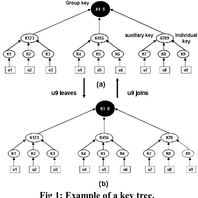
In a key tree, the root is the group key, leaf nodes are individual keys, and the other nodes are auxiliary keys. Consider a group of 9 user’s u1... u9. A key tree of degree 3 is shown in Figure 1(a).The Key server follows three strategies to distribute the new keys to the remaining users: user-oriented, key-oriented, and group-oriented. Using group-oriented rekeying, the key server constructs the rekey message and multicasts it to the whole group.
Fig 1: Example of a key tree.
From the above example, we can see that both the server’s computation and communication costs are proportional to the number of encryptions to be performed (5 for the first example and 4 for the second example). Thus, we use server cost to mean the number of encryptions the key server has to perform. If the key tree degree is d and there are N users, assuming the key tree is a completely balanced tree, the server cost is 2 log d N for a join and d log d N -1 for a leave.
2.2 Key Star
every user’s individual key, puts the encrypted keys in a message and multicasts it to the whole group. Clearly, using a key star, the server cost is 2 for a join and N -1 for a leave.
Fig 2: Example of a key star.
3. INDIVIDUAL REKEYING
Ideally, a departed user should be expelled from the group, and a new user be accepted to the group, as early as possible. Thus, the key server should rekey immediately after receiving a join or leave request, we call this individual rekeying. Individual rekeying, however, has two problems: Inefficiency and an out-of-sync problem between keys and data.
3.1. Inefficiency
Individual rekeying is relatively inefficient for two reasons. First, the rekey message has to be signed for authentication purpose; otherwise a compromised group user can send out bogus rekey messages and mess up the whole system. Signing operation is computationally expensive. If, for every single request, the key server has to generate and sign a rekey message, the signing operation alone will place a heavy burden on the key server, especially when requests are frequent.
Second, consider two leaves that happen one after another. The key server generates two sets of new keys (group key and auxiliary keys) for these two leaves. These two leaves, however, might temporally happen so close to each other that the first set of new keys are actually not used and are immediately replaced by the second set of new keys. When requests are frequent, like during the startup or teardown of a multicast session, many new keys may be generated and distributed, while not used at all. This is a waste of server cost.
3.2 Out-of-Sync Problem
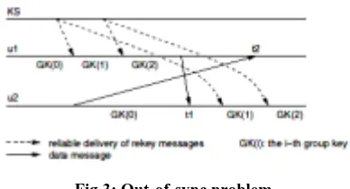
Individual rekeying also has the following out-of-sync problem between keys and data: a user might receive a data message encryptedby an old group key, or it might receive a data message encrypted with a group key that it has not received yet. Figure 3shows an example of this problem. In this example, at time t1, u2 receives a data message encrypted with group key GK(2) from u1, but u2 has not received GK(2); at time t2, u1 receives a data message encrypted with group key GK(0) from u2, but u1’s current group key is GK(2). Delay of reliable rekey message delivery can be large and variable. Thus, this out-of-sync problem may requirea user to keep many old group keys, and/or buffer a large amountof data encrypted with group keys that it has not received.
Fig 3: Out-of-sync problem
4. BATCH REKEYING
To address the above two problems, we propose the use of periodic batch rekeying[1]. In batch rekeying, the key server waits for a period of time, called a rekey interval, collects the entire join and leave requests during the interval, generates new keys, constructs a rekey message and multicasts the rekey message. Batch rekeying improves efficiency because it reduces the number of rekey messages to be signed: one for a batch of requests, instead of one for each. Batch rekeying also takes advantage of the possible overlap of new keys for multiple rekey requests, and thus reduces the possibility of generating new keys that will not be used.
5. MARKING ALGORITHM
Marking algorithm for the key server to process a batch of requests. Obviously, if the key server uses key star, batch rekeying is a straightforward extension to individual rekeying. Thus, the marking algorithm applies to key tree only. We analyze the resulting server processing cost for batch rekeying. We use J to denote the number of joins in a batch and L to denote the number of leaves in a batch. We assume that within a batch, a user will not first join then leave, or first leave then join.
5.1 Marking Algorithm
Given a batch of requests, the main task for the key server is to identify which keys should be added, deleted, or changed. In individual rekeying, all the keys on the path from the request location to the root of the key tree have to be changed. When there are multiple requests, there are multiple paths. These paths form a subtree, called rekey subtree, which includes all the keys to be added or changed. The rekey subtree does not include individual keys. The key server cannot control which users might leave, but it can control where in the key tree to place the new users. Thus, the key server should carefully place the new users (if there were any) so that the number of encryptions it has to perform is minimized.
The algorithms as follows
Case 1: J = L.
1. Replace leaves by joins.
2. Mark all the nodes from the replacement locations to the root UPDATE.
Case 2: J < L
1. Out of the L leaves, pick J shallowest (smallest height) leaves. 2 Replace these J leaves with the J joins.
Those leaving nodes without joining
replacements are marked DELETE. A non-leaf node is marked DELETE if and
only if all of its children are marked DELETE.
Case 3: J > Land L = 0.
1. Find a shallowest leaf node v. Remove v from the tree.
2. Construct T, a complete but not necessarily balanced tree [11], that has all the new users and v as leaf nodes. The other nodes of T are new keys.
3. Attach T to the old location of v.
4. Mark all T’s internal nodes NEW and mark all the nodes from the root to the parent of v’s old location UPDATE.
Case 4: J > Land L > 0. 1. Replace all leaves by joins.
2. Find a shallowest leaf node, v, among the replacement locations. Remove V from the tree. 3. Construct a complete tree T that has the extra joins and v as leaf nodes. The other nodes of T are new keys.
4. Attach T to the old location of v.
5. Mark all T’s internal nodes NEW and mark all the keys from the replacement locations (except the old location of v) to the root UPDATE.
After marking the key tree, the key server removes all nodes that are marked DELETE. The nodes marked UPDATE or NEW form the rekey subtree. The key server then traverses the rekey subtree, generates new keys, encrypts every new key by each of its children, constructs and multicasts the rekey message. It is not hard to see that the running time of the marking algorithm is O ((J + L) logd N + N).
5.2 Keeping the Key Tree Balanced
To achieve best performance, a key tree should be kept more or less balanced. Our marking algorithm aims to keep the tree balanced across multiple batches, by adding extra joins to the shallowest leaf node of the tree in each batch. However, depending on the actual locations of the requests, even if the key tree starts complete and balanced, it is possible that the key tree may grow unbalanced after some number of batches. For example, many users located close to each other in the key tree may decide to leave at the same time. It is impossible to keep the key tree balanced all the time, without incurring extra cost.
6. 2-3 TREE or B-TREE (of order m=3)
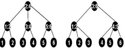
Definition: A 2-3 tree is a tree in which each vertex which is not a leaf has 2 or 3 sons, and every path form the root to a leaf is of the same length. Note that the tree consisting of single vertex is a 2-3 tree. Let T be a 2-3 tree of height ‘h’. The number of vertices of T is between 2h+1-1 and (3h+1-1)/2, and the number of leaves is between 2h and 3h.
Fig 4: Examples for 2-3 Trees.
A 2-3 tree can represent a linearly ordered set S by assigning the elements of the set to the leaves of the tree. We can use E[l] to denote the element stored at leaf ‘l’. We can use 2-3 trees to implement dictionaries (Insert, Delete, Member), Priority Queue (Insert, Delete, Min), Mergable Heap (Insert, Delete, Union, Min), Concatenable Queue (Insert, Delete, Find, Concatenate, Split). Depends on the application we assign the elements of set to leaves of the tree. For ex: In case dictionary, we assign the elements in increasing order from left to right. At each vertex ‘v’ which is not a leaf, we need two additional pieces of information. L [v] and M [v]. L [v] is the largest element of S assigned to the sub tree whose root is the leftmost son of v; M [v] is the largest element of S assigned to the sub tree whose root is the second son v. The values of L and M attached to the vertices enable us to start at the root and search for an element in a manner analogous to binary search. The time to find any element is proportional to the height of the tree (h=O (logn)). In all other cases no restriction in order to assign the elements as leaves.
6.1 Insertion of new element into a 2-3 Tree
To insert a new element ‘a’ into a 2-3 tree we must locate the position for the new leaf ‘l’ that will contain ‘a’. This is done by trying to locate element a in the tree. Assuming the tree contains more than one element, the search for ‘a’ terminates at a vertex ‘f’ such that ‘f’ has either two or three leaves as sons.
If ‘f’ has only two leaves l1 and l2, we make ‘l’ a son of ‘f’. If a < E[l1], we make l the leftmost son of ‘f’ and set L[f]=a and M[f]=E[l1]; if E[l1]<a<E[l2], we make l the middle son of ‘f’ and set M[f]=a; if E[l2]<a, we make ‘l’ the third son of ‘f’. The L and M values of some proper ancestors of ‘f’ may have to be changed in the latter case. Now suppose ‘f’ already has three leaves, l1, l2, and l3. We make ‘l’ the appropriate son of ‘f’. Vertex ‘f’ now has four sons. To maintain the 2-3 tree property, we create a new vertex ‘g’. We keep the two left most sons as sons of ‘f’, but change the two right most sons into sons of ‘g’. We then make ‘g’ a brother of vertex ‘f’ by making ‘g’ a son of the father of ‘f’. If the father of ‘f’ had two sons, we stop here. If the father of ‘f’ had three sons, we must repeat this procedure recursively until all vertices in the tree have at most three sons. If the root is give four sons, we create a new root with two new sons, each of which has two of the four sons of the former root.
Algorithm 6.1: Insertion Operation
Step 2: If T has more than one vertex, let f=SEARCH (a, r), where SEARCH is the procedure described in successive algorithms. Create a new leaf ‘l’ labeled ‘a’. If ‘f’ has two sons labeled b1 and b2, and then make ‘l’ the appropriate son of ‘f’. Make ‘l’ the left son if a<b1, the middle son if b1<a<b2, the right son if b2 <a. If ‘f’ has three sons, make ‘l’ the appropriate son of ‘f’ and then call ADDSON (f) to incorporate ‘f’ and its four sons into T. ADDSON is the procedure described next. Adjust the values of L and M along the path from ‘a’ to the root to account for the presence of ‘a’.
Algorithm 6.2 SEARCH (a, r) {
if any son of r is a leaf then return r; else
{
let si be the ith son of r;
if a<=L[r] then return SEARCH (a, s1);
else
if r has two sons or a<=M[r] then return SEARCH(a, s2);
else
return SEARCH(a, s3);
} }
Algorithm 6.3 ADDSON (v) {
create a new vertex v';
make the two rightmost sons of v the left and right sons of v';
if v has no father then {
create a new root r;
make v the left son and v' the right son of r; }
else {
let ‘f’ be the father of v;
make v' a son of ‘f’ immediately to the right of v;
if ‘f’ now has four sons then ADDSON(f); }
}
Fig 5: (a) 2-3 Tree before insertion.
(b) 2-3 Tree after inserting 3 in fig 9 a.
Fig5: continues (c) 2-3 Tree after inserting 4 in 5a.
6.2 Deletion operation
An element ‘a’ can be deleted from a 2-3 tree in essentially the reverse of the manner by which an element is inserted. Suppose element ‘a’ is the label of leaf ‘l’. There are three cases to consider.
CASE 1: If ‘l’ is the root, remove ‘l’.
CASE 2: If ‘l’ is the son of a vertex having three sons, remove ‘l’.
CASE 3: If ‘l’ is the son of a vertex ‘f’ having two sons ‘s’ and ‘l’, then there are two possibilities:
(a). ‘f’ is the root. Remove ‘l’ and ‘f’, and
leave the remaining son ‘s’ as the root.
(b). ‘f’ is not the root. Suppose ‘f’ has a brother ‘g’ to its left. A brother to the right is handled similarly. If ‘g’ has only two sons, make ‘s’ the right most son of ‘g’, remove ‘l’, and call the deletion procedure recursively to delete ‘f’. If ‘g’ has three sons, make the right most son of ‘g’ be the left son of ‘f’ and remove ‘l’ from the tree.
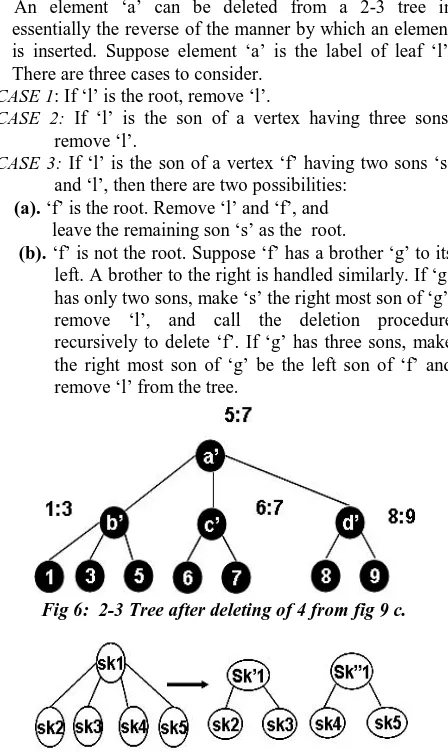
Fig 6: 2-3 Tree after deleting of 4 from fig 9 c.
Fig 7: Node sk1 splits into nodes sk1' and sk1". B-tree
order m=3.
6.3 Splitting One Node Costs m+1 Multicast Messages
sk1" know sk1, which gives them the ability to trace the subgroup keys from sk1' (=sk1) up and eventually to get the group key, even if, later on, they leave the group. To achieve further confidentiality, the server could change sk1' =sk1) when a member in the subgroup sk1" leaves. However, since sk1' (=sk1) is not on the path from the root to the members in sk1", changing sk1' (=sk1) requires the server to remember which keys out of the path are known by the members in the subgroup sk1". This causes the rekeying procedure to become complicated and may raise the rekeying cost to as high as n (when a leaving member knows many subgroup keys out of the path).
Following nodes splitting, the new subgroup keys sk1' and sk1" are distributed in four multicast messages, sk2{sk1 sk1'}, sk3{sk1 sk1'}, sk4{sk1 sk1"}, and sk5{sk1 sk1"}. Notice that we can’t use sk1{sk1 sk1'}and sk1{sk1 sk1"} because the members in the subgroups sk1' and sk1" know sk1 and can decrypt both messages. Therefore, splitting one node requires m+1 multicast message. Since insertion may split up to h nodes and a unicast message of size h is used to tell the new member the subgroup keys, the worst-case rekeying cost for inserting a new member is (m+2)h.
7. NSBHO (NON-SPLIT BALANCING HIGH-ORDER) TREE
In this section, we first give the definition of the NSBHO tree[2], then, we compare the height of the NSBHO tree with that of the standard B-tree of the same order. The algorithm for inserting an external node into the NSBHO tree and removing an external node from NSBHO tree is discussed in next successive sections.
We call the nodes for group member’s external nodes. Square nodes are external nodes and all other nodes are internal nodes. We define the level of node ‘x’ as x.level=x.parent.level+1 and root. Level=0. Assuming that ‘h’ is the height of the tree (the external nodes are excluded), then the external nodes are at level ‘h’. In following figure, the external nodes are at level 3 and the tree height is 3.
Fig.8: An NSBHO tree of order 3. The shaded nodes are in the special path (SP). The tree height h=3(the external
nodes are excluded).
Definition: An empty tree is an NSBHO (Non-Split
Balancing High-Order) tree of order m. A tree with only one external node and no internal nodes is an NSBHO tree of order m. If an NSBHO tree of order m is not empty and has more than one external node, it has the following properties (d =m/2):
P1. The root has at least two children and at most m children.
P2. All external nodes are at the same level.
P3. All internal nodes other than the nodes in special path (defined below) and the root have at least d children and at most m children.
P4. There is at most one special path.
P5. A special path (SP) is a sequence of internal nodes, (z0,
z1, . . . , zk), where zi is an ancestor of zi-1 for 0<= i < k, zi
has at least one child and at most d-1 children for 0<= i<= k, and z0 is not the root.
Above figure. 8 give an example of an NSBHO tree of order 3. The shaded nodes are in special path. Node z0 is the parent certainly an ancestor, of node z1. The difference between the NSBHO tree and the standard B-tree is that the NSBHO tree is not a search tree and it allows a special path on which the nodes do not satisfy the property of a standard B-tree node.
7.1. Height of the NSBHO Tree
Lemma 1.Let h be the height of an order-m NSBHO tree, n be the number of external nodes, and d =m/2 .
1. mh >= n >=dh-1+ 1, 2. logd(n-1) +1>=h>= logmn.
Proof. We first prove the upper bound on n. Level 0 has one node, level 1 has at most m nodes, level 2 has at most m2 nodes, . . . , level i has at most mi nodes. Hence, there are at most mh external nodes.
Now, we prove the lower bound on n. Level 0 has one node. We claim that level i (i > 0) has at least di-1+1 node. We prove this claim by induction. Since the root is never in the special path, level 1 has at least two nodes. Assume level i-1 has at least di-2+1 node. At most one of them may be in the special path (Definition 1). The nodes not in the special path have at least d children per node. Thus, level i has at least d i-1
+1 nodes. This proves the lower bound on n. The bound on h follows the bound on n.
Lemma 2.Let h be the height of an order-m B-tree, n be the number of external nodes, and d=m/2 .
1.mh >= n >= 2dh-1, 2.logd(n/2)+1>=h>=logmn.
Proof. It is easy to see that mh>= n since each internal node can have at most m children. Since all the internal B-tree nodes except the root have at least d children and the root has at least two children, the minimum number of nodes at level 0, 1, 2, 3, . . . , h is 1, 2, 2d, 2d2, . . . , 2dh-1, respectively. Therefore, there are at least 2dh-1 external nodes. The bound on h follows the bound on n.
7.2. Insert an External Node
Fig.9: An external node z is inserted into the NSBHO tree specified in 4.1 using the insertion point. (a) z0, (b ) z1, (c )
root. The resulting trees at (a) and (c) are not NSBHO trees. The resulting tree at (b), however, is an NSBHO tree.
The key is to find a suitable insert point (internal node) such that the resulting tree is still an NSBHO tree. When the special path SP is not empty, a node belongs to SP with the largest level is the suitable insert point. Recall that x.level=x.parent.level+1 and root. level=0. In Fig 13, the special path is (z0 , z1 ), z0.level=1, and z1.level=2, thus z1 is the suitable insert point. Fig. 13b shows the resulting tree using z1 as the insert point. One may verify that it is an NSBHO tree. z0 can’t be used as the insert point because, otherwise, the resulting tree (as shown in Fig. 13a) has two special paths, (z1) and(x0).The root can’t be used as the insert point either because, otherwise, the resulting tree (as shown in Fig. 13c) has two special paths, (z0,z1) and (x0 , x1 ). When the special path SP is empty, an arbitrary internal node that has fewer than m children can be the insert point. When all the internal nodes are full (i.e., having m children each), a new root will be created which becomes the insert point.
The algorithm for inserting an external node z is listed here. If the tree is empty, z becomes the root. Otherwise, getInsertPoint algorithm is invoked. If getInsertPoint returns null, a new root y is created and the current root becomes a child of the new root. Now, y has fewer than m children. A chain of internal nodes (x0, x1, . . ., xl ) is created , where xi=xi+1.parent for 0<=i < l, x0.level=y.level+1, and xl.level=h-1. The purpose of the chain is to put z at the correct level of the external nodes. The new external node z becomes a child of xl and x0 becomes a child of y. In the case of y.level=h-1, there is no need to create a chain and, thus, z itself becomes a child of y. getInsertPoint algorithm returns null if there is no internal node or all internal nodes are full. If SP is not empty, a node belongs to SP with the largest level is returned. Otherwise, a nonfull internal node does not belong to SP is returned.
Special Path (SP) can be maintained by a simple array of size h. Adding (removing) a node to (from) SP can be done in O(1) time. Returning the node belongs to SP with the largest level is the key to making the insertion algorithm work.
Algorithm for inserting an External Node ‘z ‘, where ‘z’ is an external node.
Algorithms 7.1 insert (TreeNode z) {
If (root==null){root=z;return;} TreeNode y=getInsertPoint (); If(y==null)
{ y=new TreeNode;
The Current root becomes a child of y;
root=y; }
create a chain of nodes as described; attach z to the end of the chain; The root of this chain becomes a child of y;
}
Algorithm 7.2 getInsertPoint ()
{ If(no internal node or all internal nodes are full)
return null;
if(SP is not empty)
return the node belongs to SP with the largest level; return an arbitrary non-full
internal node does not belongs to SP.
}
7.3. Remove an External Node
No rebalancing is needed after an external node z is removed if the parent of z is not one child short (i.e., if z.parent is in SP, z.parent should have at least one child and, if z.parent is not in SP, z.parent should have at least d children). The tree rebalancing is carried out only when z.parent is one child short. If z.parent is in SP, “one child short” means z.parent has no children left and, thus, z.parent can be removed, which causes z.parent.parent to lose a child. We need to move one level up the tree and check z.parent.parent to see whether or not rebalancing is necessary there. If z.parent is not in SP, we will use the standard B-tree technique (i.e., borrowing a child from sibling or merging z.parent with its sibling). If it is possible for z.parent to borrow a child from its sibling, rebalancing ends. Merging z.parent with its sibling causes z.parent.parent to lose a child. Thus, we need to move one level up and check z.parent.parent. Due to the existence of SP, z.parent.parent may have only one child. In this case, borrowing or merging is not possible. However, we can add z.parent to SP without violating the NSBHO property and there by terminating the rebalancing.
Algorithm for removing a ‘z’, where ‘z’ is an external node.
Algorithms 7.3 remove (TreeNode z) { If(z==root) { root=null; return;} TreeNode pz=z.parent;
pz.removeChild (z); z=pz;
while (z!=root and (z.size==d-1 or z.size==0))
{ pz=z.parent; if(z belongs to SP)
{ remove z from SP; pz.removeChild(z); delete z; z=pz;
else{ TreeNode sz=richSibling(z); If(sz exists)
{move a child from sz to z; z=root;} if(pz.size>1)
{ Merge z with a sibling of z; z=pz; } else
{ Add z to SP; z=root;} }
}
if(z==root and z.size <2 ) {root= the only child of z; if(root belong to SP)
remove root from SP; }
}
Algorithm 7.3 describes the procedure for removing an external node ‘z’. The siblings of ‘z’ include all the children of z.parent except z. The function richSibling(z) returns a sibling of sz of ‘z’ such that (sz belongs to SP and sz.size >1) or (sz does not belongs to SP and sz.size >d ). However, if no such sz exists, richSibling(z) return null.
The while loop is executed when z is an internal node, z is not the root, and z is one child short (deficiency). If z is in SP , “one child short” means z has no child, thus z can be deleted. If z is not in SP , “one child short” means z has d-1 children. The deficiency can be compensated for by borrowing a child from the sibling of z if z has a rich sibling, by merging with a sibling if z has at least one sibling, or by adding z into SP if z has no sibling. The deficiency may propagate one level up, thus we need to move one level up to check the parent of z. In other cases, we terminate the while loop by setting z to the root. If the deficiency propagates up to the root, the tree height is decreased by one.
8. ANALYSIS
We analyze the server processing cost for batch rekeying. We consider the worst case and average case and compare batch rekeying against individual rekeying.
Key star’s batch rekeying server cost, denoted as RB (N, J, L) is:
{
(
1 00
)
,
,
=
JN++JifL−LifL= >B
N
J
L
R
Thus, our analysis mainly focuses on key trees. For the purpose of analysis, we assume that the key tree is a complete and balanced tree at the beginning of a batch, and that each current user has equal probability of leaving. Let d be the key tree degree, N be the group size at the beginning of a batch, h be the height of the key tree (h = logd N), W(N,d,J, L) be the worst case batch rekeying server cost, and E(N,d,J, L) be the average case batch rekeying server cost.
8.1 Worst Case Analysis
The marking algorithm can control where to place joins, but cannot control where leaves happen. Thus, worst case analysis mainly considers how the locations of leaves affect the server cost. Since the marking algorithm takes different operations for four cases, worst case analysis is also divided into four cases.
Case 1: J = L.
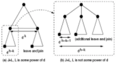
For simplicity, we first assume L = d k for some integer k. When J = L, the worst case happens when the leaves are evenly distributed across the N leaf nodes in the key tree. The server cost for this case is:
(
)
(
)
1
1
,
,
,
−
−
+
=
=
d
L
d
L
N
LdLog
L
J
d
N
W
dIf L is not some power of d, suppose L = dk + r, 0 < r < (d - 1) dk, then in the worst case, each of the r additional leaves adds d (h - k - 1) to the total cost
Thus,
(
)
(
)
(
)
(
1)
1 1 ,
,
, 1 + − −
− − + − =
= + rdh k
d d d k h d L J d N W k k
In other words, if dk < L < dk+1, W= (N, d, J, L) grows linearly between W= (N, d, J, dk) and W= (N, d, J, dk+1).
Fig 10: Worst case analysis.
Case 2: J < L
The analysis for this case is similar to the previous case. The only difference is that there are only N - (L - J) users left in this case. Thus,
W < (N, d, J, L) = W = (N, d, L, L) - (L - J)
Case 3: J > Land L = 0.
In this case, the marking algorithm has full control of the server cost. It is not hard to see that a complete d- ary
tree with n leaves is of size − − 1 1 d
dn ,Thus, T’s size is
(
)
− − + 1 1 1 d Jd and there are log
d N + 1 nodes from the root
to v. Thus:
(
)
N
d
dJ
O
J
d
N
W
2
log
d1
,
,
,
+
−
=
>
Case 4: J > Land L > 0.
When there are more joins than leaves, the analysis is a combination of cases 1 and 3. Thus:
8.2 Average Case Analysis
The server cost depends on the number of nodes belonging to the rekey subtree, and the number of children each node has. Thus, our technique for average case analysis is to consider the probability that an individual node belongs to the rekey subtree, and to consider the node’s expected number of children. Again, we consider the following four cases.
Fig 11: Average case analysis.
Case 1: J = L.
This case forms the basis of our analysis for the other cases. Let the root of the key tree be at level 0, and the leaf nodes be at level h, where h = logd N. Let T(x) be the sub tree rooted at node x and L(x) be the leaf nodes of T(x). Consider a node v at level, 0 <= l <= h - 1 (see Figure 19). V belongs to the rekey sub tree if and only if there is at least one leave in L (v). Assuming every current user has equal
probability of leaving, there are
{
NL ways to pick L leaving users out of N users. Among these many ways,(
N dl)
LN
−
/ of them have no leaves in L(x). Thus, the probability that v belongs to the rekey sub tree is(
)
( )
−
−
N L d N L lN
/1
Therefore,(
)
(
( )
)
−
−
=
=
∑
−= LN
d N L h l l l
N
d
d
L
J
d
N
E
/ 1 01
,
,
,
Case 2: J < L
When J < L, we should take into account the probability that some nodes might be marked DELETE and pruned from the tree. A node v is pruned if and only if all nodes in L(v) are leaves and none of them are replaced by joins. Using a similar technique as the previous case, we know the probability that a node at level l is pruned is
(
)
( )
(
( )
)
( )
( )
N d N J L d N L J d N J N L d N N d N L l l l l lL
/ / / / /.
− − −−
=
Thus(
)
(
)
∑
( )
= −−
=
=
<
h l N d N J L d N l l ld
L
J
d
N
E
L
J
d
N
E
0 / /,
,
,
,
,
,
Case 3: J > L and L = 0.
For this case,
E> (N, d, J, 0) = W > (N, d, J, 0)
Case 4: J > L and L > 0.
The analysis for this case is a combination of cases 1 and 3.Thus:
(
)
(
)
− − + = = > 1 ) ( , , , , , , d L J d L L d N E L J d N E8.3 Batch vs. Individual Rekeying
In this section, we show that batch rekeying saves server cost substantially over individual rekeying. The actual save depends on whether the key server uses key star or key tree.
8.3.1 Key Star
Let RI (N, J, L) be the cost for processing J joins and L leaves individually. Clearly,
(
,
,
)
{
(2 1)0 2 0= > + −
=
JifL JifL L NI
N
J
L
R
Thus, the difference between batch rekeying and individual rekeying is:
(
)
(
)
{
1 00 ) 1 (
,
,
,
,
−
B=
JN−LifL−=+JifL>I
N
J
L
R
N
J
L
R
The difference is substantial, especially when J and L are large.
8.3.2 Key Tree
We have mentioned that using key tree for individual rekeying; the server cost is d logd N - 1 for a leave and 2 logd N for a join.
Let S (N, d, J, L) be the server cost for rekeying a batch of J joins and L leaves individually. Clearly,
S (N, d, J, L) = (dL + 2J) logd N – L
9. RESULTS
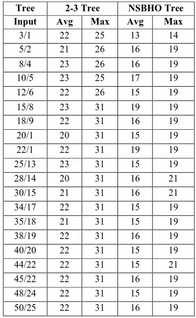
9.1 Table: Comparison Results for various inputs. (Assuming initial size of the tree 1000).
(Note: Inputs (i/p): a/b refers among ‘a’ operations,
b no. of insertions and a-b deletions).
Tree 2-3 Tree NSBHO Tree
Input Avg Max Avg Max
9.2. Graphs
Btree Order 3
14 16 18 20 22 24 26 28 30 32
0 5 10 15 20 25 30 35 40 45
Operations
R
e
ke
yi
n
g
m
e
s
s
a
g
e
co
s
t
Average costs Maximum costs
( a ) 2-3 Tree(B-Tree of order 3) Re keying Message Costs for 50 Random Insertions (50%) / Deletions (50%). Initial Tree Size is 1000.
NSBTree Order 3
14 16 18 20 22 24 26 28 30 32
0 5 10 15 20 25 30 35 40 45
Ope rations
R
e
ke
y
in
g
m
e
ssa
g
e
c
o
st
Average costs Maximum costs
( b ) NSBHO Tree of order 3.Re keying Message Costs for 50 Random Insertions (50%) / Deletions (50%). Initial Tree Size is 1000.
10. CONCLUSION
This paper addressed the scalability problem of group key management [1][2]. We identified two problems with individual rekeying: inefficiency and an out-of-sync problem between keys and data. We proposed the use of periodic batch rekeying to improve the key server’s performance and alleviate the out-of-sync problem. We devised a marking algorithm for the key server to process a batch of join and leave requests, and we analyzed the key server’s processing cost for batch rekeying. Our results show that batch rekeying, compared to individual rekeying, saves server cost substantially. We also show that when the number of requests is not large in a batch, four is the best key tree degree; otherwise, key star outperforms small-degree key trees. The hierarchical key-tree approach is an efficient way to achieve logarithmic rekeying costs for secure multicast key management given that the underlying tree is balanced. We have developed an NSBHO tree. Unlike the B-tree scheme [10], our NSBHO tree does not use node splitting to balance the tree. As a result, the worst-case rekeying cost of our NSBHO tree for a new member joining is 2h, while that of the B-tree scheme is (m+2)h, where h is the corresponding tree height and m is the order of the tree. For a member leaving, the B-tree scheme and our NSBHO-tree scheme have the same worst case rekeying cost. Our results confirm that the NSBHO tree is superior to the B-tree in
terms of the worst-case rekeying performance. In addition, it has better average-case rekeying performance.
REFERENCES
[1] Haibin Lu: A Novel High-Order Tree for secure multicast key management. IEEE Transactions on Computers, vol 54, No. 2, Feb 2005.
[2] Xiaozhou Steve Li,Yang Richard Yang,Mohamed G.Gouda,Simon S.Lam: Batch Rekeying For Secure Group Communication. ACM Paper, May 2001.
[3] A.Ballardie. Scalable Multicast Key Distribution, RFC 1949, May 1996
[4] H.Harney, C. Muckenhirn, and T.Rivers. Group key management protocol architecture, RFC 2094, July 1997.
[5] H.Harney, C. Muckenhirn, and T.Rivers. Group key management protocol specification, RFC 2093, July 1997.
[6] M.J.Moyer, J.R.Rao, and P.Rohatgi. Maintaining Balanced Key Trees for secure multicast, INTERNET-DRAFT, June 1999.
[7] D. Wallner, E.Harder, and Ryan Agee. Key Management for Multicast: Issues and Architectures, INTERNET-DRAFT, September 1998.
[8] David Balenson, David McGrew, and Alan Sherman. Key Management for Large Dynamic Groups: One-way Function Trees and Amortized Initialization, INTERNET-DRAFT,1999.
[9] Key Management for Multicast: Issues and Architectures, RFC 2627, Sep 1999.
[10] Li,Yang,Gouda,Lam. Batch Rekeying for secure group communications,www10, May 1-5,2001,Hong Kong.
[11] J.Goshi and R.E.Ladner, Algorithms for Dynamic Multicast Key Distribution Trees, Proc. ACM Symp. Principles of Distributed Computing (PODC), 2003.
Authors Biography
Ramesh Kumar .P received B.Tech (CSE), M.Tech (CSE). He is currently serving as Sr.Lecturer in the Department of Computer Science and Engineering, V.R.Siddhartha Engineering College. His research interest lies in the area of Ear Biometrics and Cryptography, Parallel Computing and Key Management. Member of CSI, IETE and ISTE.
P. Srinivasulu received his B.Tech(ECE),