Themed Section : Engineering and Technology
Selection of Deep Borehole from South and Central Australia to
Reconstruct Last Glacial Maximum Temperature History
Asadusjjaman Suman1,2 and Farnaz Akther3
1 Institute for Applied Ecology, University of Canberra, Canberra, Australia
2 Department of Agricultural Engineering, Patuakhali Science and Technology University, Patuakhali, Bangladesh
3 Faculty of Science and Technology, University of Canberra, Canberra, Australia Correspondence to: Asadusjjaman Suman ([email protected])
ABSTRACT
We analysed six deep boreholes temperature data from southern and central Australia to understand downhole temperature characteristics for inversion and to reconstruct Last Glacial Maximum (LGM) temperature histories. Analysis shows, most of the deep boreholes are not suitable for inversion to reconstruct long term temperature history. Variation in the sub-surface lithology is the main driver for not picking up climate signal from these boreholes. However, borehole is drilled in homogeneous lithology shows promise to reconstruct long term temperature history. Blanche 1 borehole from central Australia was identified as being of high quality, with a very low area misfit of ~0.001 m2/m, thus enabling for inversion to reconstruct temperature history since about LGM. Drill a deep borehole is a costly operation, thus it is recommended to select a deep borehole site carefully in homogeneous rock based on details survey in the sub-surface lithology.
Keywords : Boreholes, Lithology, Thermal conductivity, Central Australia
I.
INTRODUCTIONThe climate of the last glacial cycle (~100,000 years) contains periods of major natural variability, such as the intense cold of the Last Glacial Maximum (LGM), major fluctuations during subsequent deglaciation and the relative stability of the Holocene (Clark et al., 2009; Petherick et al., 2013; Reeves et al., 2013; Williams et al., 2009). Records of past climate help us to understand how the landscape, people and biotic inhabitants have come to be in their current state. Paleoclimate records are also important for understanding how global climate forcing, such as greenhouse gases are translated into the regional climates. Thus, any advancements in our knowledge of climate variability during this time period are important for understanding our past environment
and for improving the accuracy of future projections by climate models.
timing of the LGM (Barrows et al., 2002; Yokoyama et al., 2000) in the Australian region. However, there is less confidence in the magnitude of the temperature change between the LGM and the Holocene, and whether spatial variations in temperature changes match those recorded elsewhere across the globe (Otto-Bliesner et al., 2006).
Semi-arid and arid central Australia covers about 40% of mainland Australia and has long been a focus of research attention. There are limited records of long term temperature history in central Australia, as a result of the poor preservation of typical paleoclimate proxies, for example, pollen (Miller et al., 1997). Our understanding of paleoclimate in central Australia is dependent upon amino acid racemization rates in emu eggshells (Johnson et al., 1999; Miller et al., 1997), dune deposits (Fitzsimmons et al., 2007a; Fitzsimmons et al., 2007b; Rhodes et al., 2005), dust flux (Hesse et al., 2004; Williams et al., 2001), and lake records (Croke et al., 1996; Magee and Miller, 1998). Most of these records indicate that central Australia was dryer and cooler during the LGM than at present. However, numerical estimation of temperature change in the region is very limited during this time period.
Temperature reconstructions of the last 500 years in Australia have been generated from the south-west of western Australia (Appleyard 2005), Eastern Tasmania (Suman & White 2017; Suman et al. 2017), Australian continental average (Pollack et al. 2006) and for the last 2,000 years from east Australia (this thesis Chapter- IV). However, despite early attempts (Cull, 1980) temperature reconstructions during the LGM using borehole temperature data have not widely been applied in Australia, despite success in other parts of the world (Chouinard and Mareschal, 2009; Pickler et al., 2015). In this study, we analyze deep borehole temperature data from southern and central Australia, to understand the magnitude of temperature change between the LGM and Holocene, and the timing of these changes.
II.
METHODSGround surface temperature (GST) variations during the last glacial cycle are recorded by the Earth‟s subsurface (depth ≥1500 m, Pickler et al., 2015) as perturbations to the „steady-state‟ temperature profile (Chouinard and Mareschal, 2009; Mareschal and Beltrami, 1992). If there was no change in GST, then temperature increases with depth in the sub-surface thermal regime would govern only by the outflow of heat from Earth‟s interior. However, during the LGM and Holocene when GST changed significantly, downward temperature diffusion is recorded as perturbations in the semi-equilibrium thermal regime.
Theoretically the length of the past temperature history obtainable from borehole records is primarily dependent on the depth of borehole temperature record. This is because of the nature of the diffusive propagation of surface temperature changes into the crust (Beltrami et al., 1992; Beltrami and Mareschal, 1995; Chouinard and Mareschal, 2009; Mareschal and Vasseur, 1992). For periodic oscillation of GST, the amplitude of the temperature fluctuation decreases exponentially with depth over a length scale δ (skin depth) proportional to the square root of the period
√ , where k is the thermal diffusivity of rock, ≈ 10-6 m2s-1. This damping eliminates the high-frequency variability that is seen in meteorological records and contains long-term climatic trends in the ground temperature signal (Beltrami and Mareschal, 1995; Pickler et al., 2016).
∫
∫ ( )
Where T0 is the reference GST (steady-state temperature), Q0 is the reference heat flux (steady-state heat flux), λ(z) is the thermal conductivity, Z is the depth, H is the heat generation and is the temperature perturbation at depth Z as a result of time-varying changes to the surface boundary condition and is the thermal resistance to depth Z.
Temperature perturbations were calculated for each depth where borehole temperature measurements were available. By using the information of temperature perturbation throughout the borehole, we were able to reconstruct past GST history. We used a Matlab program that applies SVD methods (Clauser and Mareschal, 1995; Menke, 1989) to reconstruct past GST history, as described in Suman et al., (2017) and Suman et al., in review (this thesis Chapter IV). This method is well established and for further details we refer the reader to Beltrami and Mareschal (1995); Chouinard and Mareschal (2007); Chouinard and Mareschal (2009); and Mareschal and Beltrami (1992).
We assessed the reliability of each borehole temperature inversion using a range of criteria. These include the potential for non-climatic perturbation, i.e. horizontal ground water flow, high variation in sub-surface thermal conductivity (TC) that affect the temperature profiles and thus reconstruction of past GST history. We also applied a technique to assess
borehole temperature data quality based on model misfit between measured and modelled data, which is described in Suman et al., (2017) (this thesis Chapter-III).
Data Description and Study Area
Fig 1. Study area showing deep borehole locations
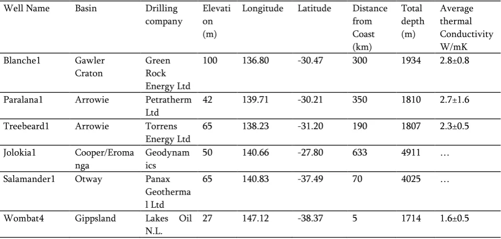
Table 1. Geologic, geographic and topographic features of deep boreholes. SiS = Siltstone, SaS = Sandstone, and CS=Claystone
Well Name Basin Drilling
company
Elevati on (m)
Longitude Latitude Distance
from Coast (km)
Total depth (m)
Average thermal Conductivity W/mK
Blanche1 Gawler
Craton
Green Rock Energy Ltd
100 136.80 -30.47 300 1934 2.8±0.8
Paralana1 Arrowie Petratherm
Ltd
42 139.71 -30.21 350 1810 2.7±1.6
Treebeard1 Arrowie Torrens
Energy Ltd
65 138.23 -31.20 190 1807 2.3±0.5
Jolokia1 Cooper/Eroma
nga
Geodynam ics
50 140.66 -27.80 633 4911 …
Salamander1 Otway Panax
Geotherma l Ltd
65 140.83 -37.49 70 4025 …
Wombat4 Gippsland Lakes Oil
N.L.
III.
RESULTS AND DISCUSSIONTo reconstruct plausible GSTH, it is important to select appropriate borehole sites (Chouinard and Mareschal, 2007). In the following section, we discuss each of the borehole sites and explain the reason behind accepting or rejecting borehole sites for use in reconstructing the temperature history of the late Pleistocene.
We calculated reduced temperature profiles (Roy et al., 2002; Roy and Chapman, 2012; Suman and White, 2017) for each borehole. Reduced temperatures were calculated from the least square fit of the thermal gradient of the lowermost part in each borehole. In reduced temperature profiles, a higher positive or negative deviation from 0oC is caused either by surface temperature change or variation in the TC. If these changes are caused by simple TC variation, then the borehole temperature profile can be corrected (Suman et al., 2017). However, in deep boreholes with complex lithology, we found that TC corrected boreholes do not yield plausible surface temperature history during inversion. This is probably caused by a lack of precise TC data throughout the borehole.
Blanche1
This hole was logged by Geoscience Associates (Australia) Pty Ltd using a normal temperature probe, a kuster geothermal temperature probe, natural gamma, density and acoustic scanner probe (Green Rock Energy Limited, 2006), and re-logged for integrated borehole temperature and other geophysical data, by the Department of State Development (DSD), South Australia.
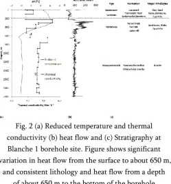
There is major lithologic variation at the top of the borehole; however, homogenous granite is present from a depth of ~650 m to the bottom of the borehole (1935m) (Fig. 2 a-c). In the granite portion, the average thermal gradient was 29.5oC/km, the harmonic mean of TC was 3.0 W/mK and the conductive heat flow, 88.5 mW/m2. Greater
variability in TC towards the top of the borehole meant that reliable temperature inversion was not detectable for the last 3000 years. The presence of consistent Pandurra and Hiltaba Suite Granite formation between 650 m and 1935 m (Fig. 2c) with very low area misfit 0.001 m2/m between measured and modelled data enabled a plausible estimate of the temperature variation between LGM and Holocene, to be determined.
Fig. 2 (a) Reduced temperature and thermal conductivity (b) heat flow and (c) Stratigraphy at Blanche 1 borehole site. Figure shows significant variation in heat flow from the surface to about 650 m,
and consistent lithology and heat flow from a depth of about 650 m to the bottom of the borehole
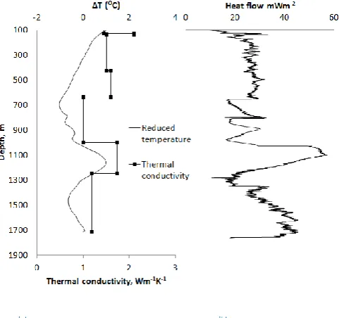
Paralana1
thermal depth temperature profile (Chouinard and Mareschal, 2009) or the past surface temperature history. Therefore, Paralana1 borehole was not used in our reconstruction of the late Pleistocene temperature history.
Fig. 3 (a) Reduced temperature and thermal conductivity (b) heat flow and (c) Stratigraphy at Paralana1 borehole site. Figure shows significant variation of lithology and heat flow throughout the
borehole.
Treebeard1
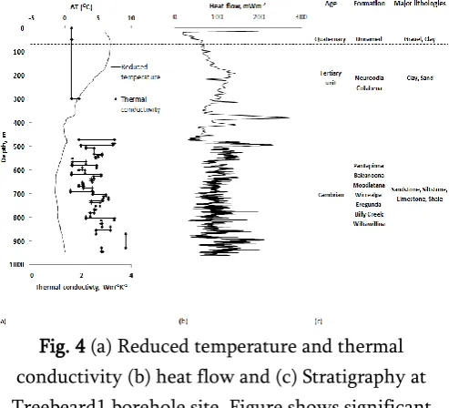
Sub-surface lithology and TC are also quite variable at the Treebeard1 borehole site (Fig. 4 a,b). Climate signal during LGM and Holocene were expected within the Cambrian unit (depth 470-1807m) of this borehole (Fig. 4c). Although the total depth of Treebeard1 is 1807 m, the temperature log is available only to a depth of 948 m and this is not enough to detect climate signal during LGM. There was also significant variability in TC values within the Cambrian unit (1.1 to 6 W/mK) and so we did not use Treebeard1 borehole data in our reconstruction of the late Pleistocene temperature history.
Fig. 4 (a) Reduced temperature and thermal conductivity (b) heat flow and (c) Stratigraphy at Treebeard1 borehole site. Figure shows significant variation of lithology and heat flow throughout the
borehole.
Jolokia1 and Salamander1
Fig. 5 (a) Reduced temperatures and (b) stratigraphy of Jolokia 1 shows significant variation in sub-surface
lithology throughout the borehole
Fig. 6 (a) Reduced temperatures and (b) stratigraphy of Salamander1 shows significant variation in
sub-surface lithology throughout the borehole.
Wombat4
There was only one borehole in Victoria that yielded enough temperature depth data to reconstruct the late Pleistocene temperature history. Wombat4 was drilled as part of a search for potential gas resources in the early Cretaceous Strzelecki group. Continuous temperature data are available from a depth of 1714 m
down to 2500 m. Sub-surface lithologies and TC are highly variable at this borehole site (Fig. 7a,b). Further, the small number of TC measurements from this borehole limits accurate TC corrections, as indicated by the high variability in the calculated heat flows with depth. The resulting inversion of raw temperature profile does not yield plausible surface temperature history. Similar results are obtained with a range of TC corrections, such as TC correction with only formation average TC values. Therefore, Wombat4 also did not use in our reconstruction of the late Pleistocene temperature history.
Fig. 7 (a) Reduced temperature and (b) heat flow at Wombat4 borehole site shows significant variation in
sub-surface lithology as well as in heat flow
Detailed analysis of six deep borehole temperature depth profiles and respective lithologies shows most of the southern and central Australian deep boreholes are not suitable for reconstructing the long-term temperature history. Only deep borehole, Blanche1, can be potentially used to reconstruct the late Pleistocene temperature history.
IV.
CONCLUSIONtemperature variation. Unfortunately, it was found most of the deep boreholes are not suitable for inversion to reconstruct long term temperature history. This is because of high variation in the sub-surface lithology. However, borehole is drilled in homogeneous lithology shows promise to reconstruct long term temperature history. Blanche 1 borehole was identified as being of high quality, with a very low area misfit of ~0.001 m2/m, thus enabling for inversion to reconstruct temperature history since about last glacial maximum. Drill a deep borehole is a costly operation, thus it is recommended to select a deep borehole site carefully in homogeneous rock based on details survey in the sub-surface lithology.
V.
AcknowledgementThe research is funded by the Australian Government Research Training Program Scholarship and Murray-Darling Basin Futures Collaborative Research Network and is part of project “Predicting the response of water quality and groundwater dependent ecosystems to climate change and land management practices: an integrated modelling approach”. We acknowledge J.C. Mareschal, Geotop, University of Quebec, Canada, for his support in base model for inversion. We acknowledge Energy Resource Division, Department of State Development, South Australia; Department of Primary Industries, Victoria for all borehole temperature and geology data.
VI.
REFERENCES
[1]. Barrows TT, Juggins S, De Deckker P, Calvo E, Pelejero C. 2007. Long-term sea surface temperature and climate change in the Australian-New Zealand region. Paleoceanography 22:1–17.
[2]. Barrows TT, Stone JO, Fifield LK, Cresswell RG. 2002. The timing of the last glacial maximum in Australia. Quat. Sci. Rev. 21:159–173.
[3]. Beltrami H, Jessop A, Mareschal JC. 1992. Ground temperature histories in eastern and
central Canada from geothermal measurements: Evidence of climatic change. Palaeogeogr. Palaeoclimatol. Palaeoecol. 98:167–184.
[4]. Beltrami H, Mareschal JC. 1995. Resolution of ground temperature histories inverted from borehole temperature data. Glob. Planet. Change 11:57–70.
[5]. Chouinard C, Mareschal JC. 2007. Selection of borehole temperature depth profiles for regional climate reconstructions. Clim. Past Discuss. 3:121–163.
[6]. Chouinard C, Mareschal JC. 2009. Ground surface temperature history in southern Canada: Temperatures at the base of the Laurentide ice sheet and during the Holocene. Earth Planet. Sci. Lett. 277:280–289.
[7]. Clark PU, Dyke AS, Shakun JD, Carlson AE, Clark J, Wohlfarth B, Mitrovica JX, Hostetler SW, McCabe a M. 2009. The Last Glacial Maximum. Science 325:710–714.
[8]. Clauser C, Mareschal JC. 1995. Ground temperature history in central Europe from borehole temperature data. Geophys. J. Int.:805–817.
[9]. Croke J, Magee J, Price D. 1996. Major episodes of quaternary activity in the lower Neales River, northwest of Lake Eyre, central Australia. Palaeogeogr. Palaeoclimatol. Palaeoecol. 124:1– 15.
[10]. Cull JP. 1980. Geothermal records of climatic change in New South Wales. Search 11:201– 203.
[11]. Fitzsimmons KE, Bowler JM, Rhodes EJ, Magee JM. 2007a. Relationships between desert dunes during the late Quaternary in the Lake Frome region, Strzelecki Desert, Australia. J. Quat. Sci. 22:549–558.
[12]. Fitzsimmons KE, Rhodes EJ, Magee JW, Barrows TT. 2007b. The timing of linear dune activity in the Strzelecki and Tirari Deserts, Australia. Quat. Sci. Rev. 26:2598–2616.
from western Tasmania, Australia. Quat. Sci. Rev. 29:2351–2361.
[14]. Green Rock Energy Limited. 2006. Blanche 1 Geothermal Exploration Hole Completion Report. West Perth WA 6872.
[15]. Hesse PP, Magee JW, van der Kaars S. 2004. Late Quaternary climates of the Australian arid zone: A review. Quat. Int. 118–119:87–102. [16]. Johnson BJ, Miller GH, Fogel ML, Magee JW,
Gagan MK, Chivas AR. 1999. 65,000 Years of Vegetation Change in Central Australia and the Australian Summer Monsoon. Science (80-. ). 284:1150–1152.
[17]. Mackenzie L, Moss P. 2014. A late Quaternary record of vegetation and climate change from Hazards Lagoon, eastern Tasmania. Quat. Int. [18]. Magee JW, Miller GH. 1998. Lake Eyre
palaeohydrology from 60 ka to the present: Beach ridges and glacial maximum aridity. Palaeogeogr. Palaeoclimatol. Palaeoecol. 144:307–329.
[19]. Mareschal JC, Jaupart C. 2011. Heat generation and transport in the Earth. Cambridge University Press, Cambridge, United Kingdom. [20]. Mareschal JC, Beltrami H. 1992. Evidence for
recent warming from perturbed geothermal gradients: Examples from eastern Canada. Clim. Dyn.:135–143.
[21]. Mareschal JC, Vasseur G. 1992. Ground temperature history from two deep boreholes in central France. Glob. Planet. Change 98:185– 192.
[22]. Menke W. 1989. Geophysical Data Analysis: Discrete Inverse Theory. International Geophysics Service.
[23]. Miller GH, Magee JW, Jull a. JT. 1997. Low-latitude glacial cooling in the Southern Hemisphere from amino-acid racemization in emu eggshells. Nature.
[24]. Otto-Bliesner BL, Brady EC, Clauzet G, Tomas R, Levis S, Kothavala Z. 2006. Last glacial maximum and Holocene climate in CCSM3. J. Clim. 19:2526–2544.
[25]. Petherick L, Bostock H, Cohen TJ, Fitzsimmons K, Tibby J, Fletcher MS, Moss P, Reeves J, Mooney S, Barrows T, Kemp J, Jansen J, Nanson G, Dosseto A. 2013. Climatic records over the past 30ka from temperate Australia - a synthesis from the Oz-INTIMATE workgroup. Quat. Sci. Rev. 74:58–77.
[26]. Pickler C, Beltrami H, Mareschal JC. 2015. Laurentide Ice Sheet basal temperatures during the last glacial cycle as inferred from borehole data. Clim. Past 12:115–127.
[27]. Pickler C, Beltrami H, Mareschal JC. 2016. Climate trends in northern Ontario and Québec from borehole temperature profiles. Clim. Past 12:2215–2227.
[28]. Rees ABH, Cwynar LC, Cranston PS. 2008. Midges (Chironomidae, Ceratopogonidae, Chaoboridae) as a temperature proxy: a training set from Tasmania, Australia. J. Paleolimnol.:1159–1178.
[29]. Rees ABH, Cwynar LC. 2010. Evidence for early postglacial warming in Mount Field National Park, Tasmania. Quat. Sci. Rev. 29:443–454. [30]. Reeves JM, Barrows TT, Cohen TJ, Kiem AS,
Bostock HC, Fitzsimmons KE, Jansen JD, Kemp J, Krause C, Petherick L, Phipps SJ. 2013. Climate variability over the last 35,000 years recorded in marine and terrestrial archives in the Australian region: an OZ-INTIMATE compilation. Quat. Sci. Rev. 74:21–34.
[31]. Rhodes E, Chappell J, Fujioka T, Fitzsimmons K, Magee J, Aubert M, Hewitt D. 2005. The history of aridity in Australia: chronological developments. Regolith:265–268.
[32]. Roy S, Chapman DS. 2012. Borehole temperatures and climate change: Ground temperature change in south India over the past two centuries. J. Geophys. Res. 117:1–12.
[33]. Roy S, Harris R, Rou R, Chapman D. 2002. Climate change in India inferred from geothermal observations. J. Geophys. Res. 107. [34]. Suman A, White D. 2017. Quantifying the
heat flow measurements. Geothermics 67:102– 113.
[35]. Turney CSM, Haberle SG, Fink D, Kershaw AP, Barbetti M, Barrows TT. 2006. Integration of ice-core, marine and terrestrial records for the Australian Last Glacial Maximum and Termination: a contribution from the OZ INTIMATE group. Quat. Sci. 21:751–761. [36]. Williams M, Cook E, van der Kaars S, Barrows
T, Shulmeister J, Kershaw P. 2009. Glacial and deglacial climatic patterns in Australia and surrounding regions from 35 000 to 10 000 years ago reconstructed from terrestrial and near-shore proxy data. Quat. Sci. Rev. 28:2398–2419. [37]. Williams M, Prescott JR, Chappell J, Adamson
D, Cock B, Walker K, Gelli P. 2001. The enigma of a late Pleistocene wetland in the Flinders Ranges, South Australia. Quat. Int. 82:129–144. [38]. Yokoyama Y, Lambeck K, De Deckker P,