MODELLING THE ACTIVITY TRAVEL PATTERN OF COMMUTERS IN A MEDIUM SIZED CITY IN INDIA

MODELLING THE ACTIVITY TRAVEL PATTERN OF COMMUTERS

IN A MEDIUM SIZED CITY IN INDIA

Parambath Koyilerian Sreela1_{, MathaVenkitachala Lakshmi Ranga Anjaneyulu}2 1 _{Government Engineering College, Calicut, Kerala, India}

2 _{National Institute of Technology, Calicut, Kerala, India}

Received 6 August 2018; accepted 1 November 2018

Abstract: This paper explores the factors influencing a worker’s decision to choose an activity pattern for commuting in a city in India. Activity and travel information collected by home interview survey formed the database for the study. Multinomial logit models were developed to understand the factors affecting the workers decision to choose an activity pattern for commute. Analysis of variance tests performed on different characteristics of the working people suggest the need for separate analysis and modelling of these categories of workers. Modelling results indicates that workers are more likely to adopt HWH pattern of work. Age, gender, presence of school students, household size, start time for work etc. were found to influence activity pattern generation of the working people. The elasticity measures were also determined to understand the influence of variables in a better way. It shows that the probability to participate in HWH activity pattern increases with unit increase in household size and school going students. The probability to participate in HWH+ increases with unit increase in employed couples in the household.

Keywords: commute, home interview, activity pattern, Calicut, India.

2_{Corresponding author: [email protected]}

1. Introduction

Activity-based approaches are the most encouraging substitute for the current travel forecasting approach. The activity based models represents the third generation of travel demand models and were in practice since the beginning of 1980’s. The development of such models has accelerated during the last 10 years, due to the increase in policy measures such as road pricing and parking pricing. In the activity based modelling concept travel is derived from a person’s entire day’s activity. It considers the interdependencies on trips and activities made by the individual. The model has been successful in explaining the reason

for selecting a particular activity pattern of travel. They also provide a fundamental and comprehensive framework to examine travel behaviour than the conventional models for forecasting travel demand. Activity based models considers activity pattern as the unit of analysis. Analysis and modelling of activity pattern are thus an essential requirement of activity based models.

constraints. Chapin’s theory concentrates on activity patterns that determine the demand for housing, employment and other facilities at particular times and places. According to McNally, (1996), travel is derived from activity participation and travel behaviour is delimited by temporal and spatial constraints on linkages between activities, locations, times and individuals. These studies resulted in identifying various types of activity patterns. The urban planning

processes shouldtherefore be based on an understanding of the determinants and evolution of activity patterns. Individuals with different activity pattern exhibit different characteristics and hence possess different travel behaviours. Therefore, it is essential to differentiate the activity pattern before evaluating their travel behaviour.

Majority of the earlier works on activity-based research were on analysing the commuting behaviour (Horner, 2004; McGuckin and Murakami, 1999; Sultana and Weber, 2014; Mao et al., 2016) and its related travel, as work activity participation and concentration are considered as the main reasons for traffic congestion during peak hours. Castro et al. (2010) observed the

influence of gender, education level, type of person, presence of children, marital status, vehicle availability, income and commute distance on worker’s propensity to make stops. (Kuppam and Pendyala, 2001), observed the strong relationships of com muter s’ soc io - demog raph ic characteristics, activity engagement information, and travel behaviour. Workers participate less in shopping and recreation due to the short time available for personal use and they spend less time these activities (Bhat et al., 2016).

An activity pattern comprises of trips and activities connected in a particular fashion. Depending on the number of locations visited within the tour or chain, activity patterns are divided into simple and complex (Ye et al., 2007). These activity patterns provide information like number of trips, travel mode, travel time, travel distance etc. A simple activity pattern involves participation in only one activity. The complex patterns are composed of more than one activity participations. Lenntorp, 1976; Adler and Ben Akiva (1979) observed activity and activity pattern generation in their works. An example of a simple activity pattern is shown in Fig.1.

Home

Office

Fig.1.

Activity pattern also signifies the sequence of activities in which an individual participates, which in turn includes locations or destinations. It thus provides the background information necessary to understand the complex interaction

among urban structure, transportation system and people’s activity participation (Xu et al.,

2009). An activity pattern of three trips and two activities is shown in Fig. 2. This is a simple case of HWSH activity pattern.

HOME

SHOP

WORK Trip 1

Trip 2 Trip 3

Fig.2.

A Complex Activity Pattern

Majority of the comprehensive models for travel demand forecast in the country were developed only in some of the metropolitan cities. In the case of medium sized cities, widespread mobility plans are rarely prepared due to scarcity of funds. These cities are also facing severe congestion due to high population growth, increased vehicle ownership and lack of good public transportation system. Hence it is very essential to explore the travel behaviour of people in such regions.

The main objective of the present study is to explore the underlying factors affecting the worker’s decision to choose an activity pattern using multinomial logit models. Another objective is to explore the need

for separate analysis and modelling of different categories of workers through the analysis of variance (ANOVA). Finally the model elasticities are also presented to offer a better understanding of influence of different variables on activity pattern generation of working people. The study has much significance as the individuals connect trips and activities in a convenient fashion to reduce travel resources and problems generated by transportation.

2. Study Area and Data Collection

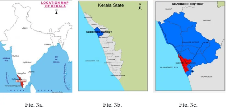
the population of Calicut corporation is 0.61 million spreads over an area of 118.59 sq. km having a population density of 5171 persons per sq. km. The city is well connected by road, rail and air. There are three national

highways (NH-17, NH-212, and NH-213) passing through the city. The total lengths of road network of the urban area are 335 km. The road density is 2.824 km per sq. km. Fig.3. shows the map of Calicut.

Fig. 3a. Fig. 3b. Fig. 3c.

Fig.3. Map of Calicut

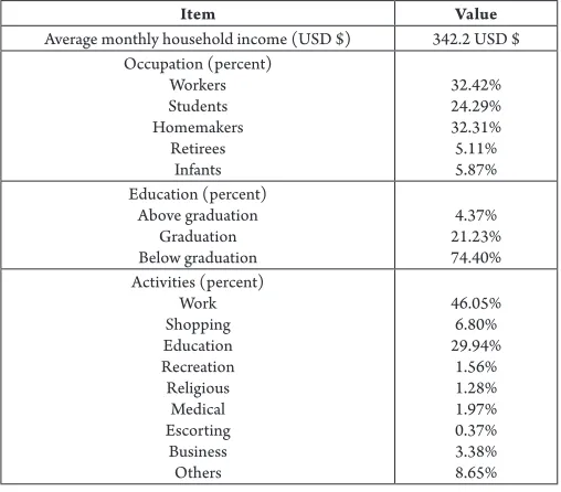
The data collection process was organized using home interview survey through an activity travel diary. The format of the diary was finalized after conducting a pilot survey. Data collection was made by trained enumerators. The activity travel information was used to include details of all activity and travel particulars. Activity and travel details of one day were collected from all members of the randomly selected households, except infants. The study used activity and details collected from 8509 workers from 9901households. An exploration of the data was done to understand the trends and patterns of the data and the general characteristics of the area. The household size varied from one to thirteen, with mean value of four. Average number of employees per household is 1.32. Male to female ratio is 0.96. Nearly 39% of households own at least one automobile and

Table 1

Sample Characteristics of Study Area

Item Value

Average monthly household income (USD $) 342.2 USD $ Occupation (percent)

Workers Students Homemakers

Retirees Infants

32.42% 24.29% 32.31% 5.11% 5.87% Education (percent)

Above graduation Graduation Below graduation

4.37% 21.23% 74.40% Activities (percent)

Work Shopping Education Recreation Religious

Medical Escorting

Business Others

46.05% 6.80% 29.94% 1.56% 1.28% 1.97% 0.37% 3.38% 8.65%

The sample is observed to be a representative of the socio-demographic trends in the study area and is comparable with the information published by census 2011 with respect to household size, gender ratio and dependency ratio. The distribution of male and female population in the sample is 49% and 51% respectively.

Different types of activity pattern were observed in the sample data. These activity patterns consist of simple and complex pattern. Majority of the individuals perform only simple activity pattern. A very less percentage (10%) of the female is found to participate in complex activity pattern. Public transportation is the most preferred mode for executing simple activity pattern. For complex activity pattern the car or two wheelers are used. This shows the flexibility of the private mode in making stops for more than one activity participation. Nearly 41% of people use public transportation for

performing simple activity pattern. Nearly 22% of the population prefer two wheelers for simple activity pattern and 38% for complex pattern.

3. Analysis of Variance

statistic, F, is calculated by comparing a ratio of the differences between the means of the groups of the variability within groups. The larger value of F represents real effects. Results are presented in the form of ANOVA table and contain the estimates of the sum of squares (SS) among, within and F-value. It also contains the associated ‘p’ value. The value of ‘p’ ranges from 0 to 1, it is the probability of calculating a given test

statistic assuming that the means of groups are identical. The larger the test statistic, lower the chance (p) that an observed difference between groups is due to chance. ANOVA tests were performed for selected variables like age, travel distance, personal income, automobile ownership and work duration.

The results are given in Table 2.

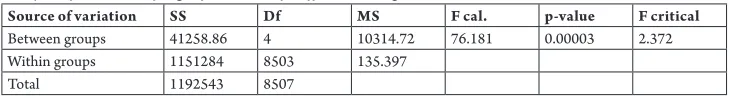
Table 2

Analysis of Variance of Age of Workers of Different Categories

Source of variation SS Df MS F cal. p-value F critical

Between groups 41258.86 4 10314.72 76.181 0.00003 2.372 Within groups 1151284 8503 135.397

Total 1192543 8507

In this case the calculated value of F is greater than the critical value hence it rejects null hypothesis. Therefore the mean age of the five groups of workers are not same. At least one of the means is different, which means that the total variation in terms of age significantly differ from at least one category of workers. With a sample size of 8508 observations, the probability that the differences between the ages of different categories of workers are due to chance only, is very less and equals 0.00003. This shows that they are significantly different from each other. The results indicate that the calculated value of F is greater than the critical value of all the cases. Therefore it is statistically confirmed that there exists variation in different categories of workers.

4. Modelling Methodology

Multinomial logit model is used for calibration process as there are more than

two alternatives. Eq. (1) shows the model form.

( ) in

jn

V

n V

j e P i

e

=

∑

Where:

Vin and Vjnare the systematic utilities of

alternatives i and j and Pn (i) is the probability

of choosing alternative ‘i’ by an individual ‘n’.

4.1. Statistical Significance of Model

The model fitness is assessed using statistical measures, namely, t-statistic, level of significance, chi-squared value, model predictability and adjusted likelihood ratio index (ρ2_{). The ratio of the departure of an}

test when it is true. Chi-squared values are the difference between initial and final log likelihood value. The initial log likelihood value is a measure of a model with no independent variables, i.e. only a constant or intercept. The final log likelihood value is the measure computed using all variables that have been entered into the model. The rho-squared value is used to describe the overall goodness of fit. It is calculated as (Ben-Akiva and Lerman, 1985) given in Eq. (2):

2 ₁ ( )

( )

LL LL c

β

ρ = − ₍₂₎

W here: LL(c) = log-likelihood for the constant only model and LL(β) = log-likelihood for the estimated model. Adjusted likelihood ratio index (ρ2_{) (Ben-Akiva and}

Lerman, 1985) is another measure for model fitness, and is given in Eq. 3:

2 ₁ ( )

( )

LL K

LL c

β

ρ = − − ₍₃₎

W here ‘K’ is the degrees of freedom (parameters) in the model.

4.2. Model Predictability

Predictability of the model is assessed based on the actual and predicted choice of each individual. The model predictability is determined using utility of the multinomial logit model.

4.3. Model Elasticity

In the case of logit transformation the sign of a parameter only indicates that the associated variable has a positive or negative influence upon the choice probabilities. There is no behavioural interpretation of a parameter estimate of a choice model, beyond the sign of a parameter. Elasticity is a unit less measure that describes the relationship between the percentage change of one variable and the dependent variable. The direct point elasticity for MNL model is given in Eq. (4):

. iq

ikq

P iq ikq

X

ikq iq

P X

X P

E

∂ (4)

The equation is interpreted as the elasticity of the probability of alternative ‘i’ for decision maker ‘q’ with respect to a marginal change in the kth _{attribute of the i}th _{alternative (ie}

X_ikq) as observed by the decision maker ‘q’. The calculation of arc elasticity involves using an average of before and after change values as indicated in Eq. (5), i.e. the above equation becomes:

. iq

ikq

ikq

P iq

X

iq ikq P X

X P

E

∂ ₍₅₎

Table 3

List of Variables for Activity Pattern Generation Variable Description of the variable

PSGC Presence of school going children in the household.1 if there are school students in the household; _{0 otherwise} HHSZ No. of members in the household

EC Employed couples

NST Number of students in the household GEN Worker’s gender 1 if male; otherwise 0

AGE Age of worker in years

SZ Location factor; 1 if the residence and workplace are in the same zone TWCH Two wheeler choice, 1 if two-wheeler is used for travel

STARTM 1 if the worker starts for work during morning 6 to 8; Otherwise STARTMP 1 if the worker starts for work during morning 8 to 10am; 0 otherwise Day of the

week Day 1, Monday; Day 2, Tuesday; Day 3, Wednesday; Day 4, Thursday; Day 5, Friday; Day 6, Saturday;

Structure of work and the various pattern

considered is shown in Table 4. The alternative 2 will be mentioned as HWH+ pattern for convenience.

Table 4

Structure of Work and Its Related Activity Pattern

Alternatives Description Activity pattern

0 Non-participation in activity

-1 Work only pattern (no non-work activities, except work related activities _{occurring during a designated day)} HWH

2 Work with additional non-work activity these include HOWH; HWOH; _{HWHOH; or HWOWH} HWH+ H-HOME; W-WORK; O-OTHER (All activities excluding work, shopping and recreation undertaken on a commute day).

5. Workers Decision to Execute an Activity Pattern

Calibration results of MNL of workers decision to choose activity travel pattern are presented in Table 5.

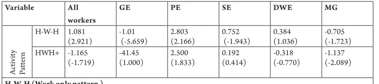
Table 5

Model Estimates for Activity Pattern Generation

Variable All

workers

GE PE SE DWE MG

Act

iv

ity

Pat

te

rn

H-W-H 1.081

(2.921) -1.01 (-5.659) 2.803 (2.166) 0.752 (-1.943) 0.384(1.036) -0.705(-1.723) HWH+ -1.165

(-1.719) -41.45 (1.000) 2.500 (1.833) 0.192 (0.414) -0.318(-0.770) -1.137(-2.089)

Variable All workers

GE PE SE DWE MG

NSTUD 0.170

(2.866) 0.201(3.074) AGE -0.017

(-3.618) -0.022(-2.520) -0.018 (-3.775) -0.021(-4.147) STARTMP 1.049

(8.234) 0.828(3.834) 1.914 (7.921) 1.169(8.913)

SZ 0.404

(2.339) 0.423(2.418) DAY4 1.224

(2.456)

DAY5 0.305

(2.066) HWH+

HHSZ -0.207

(-2.645) 0.847 (3.950)

EC 1.071

(3.671) 1.111(2.586) PSGC -0.610

(-2.704) -1.622 (-3.216) -0.61(-2.131)

GEN -0.709

(-1.820) -1.185(-5.478) 1.349(5.544) TWCH 0.660

(2.738) 1.239 (7.070) 0.875(4.110)

STARTM 0.428

(2.100) 0.867(3.659) DAY3 0.870

(3.251) 4.593(5.891) 1.528(6.093) DAY5 0.688

(2.885) 3.204(4.403) 2.377(7.763) 1.422(9.313) 1.345(5.826) Goodness of fit measures

LL (Constant) -2198.37 -1240.78 -1124.9 -3088.59 -3335.5 -2373.4 LL(Convergence) -1680.51 -658.86 -667.63 -2370.49 -2685.5 -1837.42 Chi-squared 1035.71 1163.82 914.56 1436.20 1300.0 1072.14 R2 _{0.235 0.468 0.406 0.232 0.194 0.218}

Adj R2 _{0.218 0.44 0.379 0.221 0.188 0.215}

Predicted 94.08 87.1 78.34 95.21 96.3 93.7

N 5501 850 1800 1000 900 980

Base alternative : Non participation in activity

The utility equation for HWH and HWH+ activity pattern for work activity is given in Eq. (6) and Eq. (7) respectively:

1.081 0.017* 1.049* 1.224* 4 HWH

V = − age+ startmp+ day

(6)

1.165 0.207 1.071 0.610 0.660 0.870 3 HWH

V + = − − hhsz+ ec− psgc+ twch+ day ₍₇₎

0 no work

Using the above utility equations the probability of an individual to choose an activity pattern is determined. The alternative specific constant indicates the increasing likelihood of workers in general to perform HWH activity pattern of work. Private employees are the major category performing HWH activity pattern. Presence of school going students results in fewer trips. That is, a commuter with students in the household is less likely to pursue HWH+ activity pattern, and prefer to spend more time for children after work. The influence of this variable is observed in the case of self-employed workers and the daily wage earners. Age negatively influences the HWH activity pattern of workers. The young workers are less likely to pursue HWH+, possibly due to the less household obligations than elders, a related finding was observed by Ye et al., (2007). The influence is same for the private employees, self-employed workers and the daily wage earners.

The workers starting for work in the morning peak are also likely to perform HWH pattern. Strathman et al. (1994) made a similar observation. All categories of workers except the daily wage earners and the marketing groups have the same influence on the likelihood of HWH pattern. Those workers residing and working in the same zone are likely to perform HWH activity pattern. This is true for daily wage earners and the marketing groups. Day of the week also influences the decision to choose an activity pattern. Workers are more likely to perform HWH activity pattern on Thursdays. Marketing groups prefers Fridays for HWH activity pattern. Negative coefficient of “HHSZ” indicates that commuters with more household members limit the worker to make HWH+ pattern. The negative sign indicates that the

on Wednesdays. Some of the earlier studies, (Pendyala and Pas, 1997)), have reported that there are substantial day to day variations

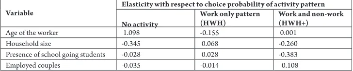
in discretionary activity participation. The Elasticities of work participation model are given in Table 6.

Table 6

Elasticities in activity generation model for workers

Variable Elasticity with respect to choice probability of activity pattern No activity

Work only pattern

(HWH) Work and non-work (HWH+) Age of the worker 1.098 -0.155 0.001

Household size -0.345 0.068 -0.260 Presence of school going students -0.028 0.028 -0.383 Employed couples -0.035 -0.014 0.108

The probability of worker to participate in HWH pattern decreases by 0.155% with one unit increase in age and the probability to participate in HWH+ pattern increases by 0.001%. The elasticity for household size indicates that the probability of workers to participate in HWH pattern increases by 0.068% with one unit increase in household size and the probability to participate in HWH+ pattern decreases by 0.26 % for one unit increase in household size.

It is also observed that the probability of workers to participate in HWH pattern decreases by 0.014 % for one unit increase in the presence employed couples and the probability increases by 0.108% for one unit increase in employed couples at home. The probability of worker to participate in HWH pattern increases by 0.028% for one unit increase in school going children and decreases by 0.383% for the same increase in school going

6. Summary

The Empirical results presented in this study demonstrate that there exists difference in activity pattern generation of different categories of workers. It explained that

personal, household; activity and travel attributes have an impact on activity pattern generation of workers. Age inf luences activity pattern of workers and the young workers are less likely to execute HWH+ pattern, similar findings was reported in other counties also (Ye et al., 2007). There are significant gender differences in activity patterns, indicating restrictions on individuals’ activity pattern generation. Influence of transportation mode and day of the week was also evident in the study.

evident from the variable representing the location of work place with respect to place of residence (SZ).

The household size of Calicut Corporation shows a decreasing trend from more than 7 in 1971 to around 4.5 in 2011. The overall trend indicates the change in joint family system to the nuclear family system (Master Plan for Kozhikode Urban Area – 2035, 2017). This decreasing trend in the household size of the years in the city indicates that in future the activity pattern is likely to become complex in future. Findings in the paper can be a major aid to the transport planners in the area as it provides valuable insights to better estimate of travel demand. Studies in this line are expected to assist planners in formulation and implementation of efficient travel demand management strategies. This database can be effectively used to explore the travel characteristics of people in Calicut city and which can be a major contribution to the study of travel behaviour in future.

Acknowledgments

We sincerely acknowledge the funding from the Ministry of Urban Development, Government of India through the Centre of Excellence (CoE) in Urban Transport, Department of Civil Engineering, IIT Madras.

References

Adler, T.; Ben-Akiva, M. 1979. A theoretical and empirical model of trip chaining behaviour, Transportation

Research Part B: Methodological 13(3): 243-257.

Ben-Akiva, M.; Lerman, S.R. 1985. Discrete choice analysis:

Theory and application to travel demand. Cambridge, MA:

MIT Press. 384 p.

Bhat, C.R.; Astroza, S.; Bhat, A.C.; Nagel, K. 2016. Incorporating a multiple discrete-continuous outcome in the generalized heterogeneous data model: Application to residential self-selection effects analysis in an activity time-use behavior model, Transportation Research Part B:

Methodological 91: 52-76.

Castro, M.; Eluru, N.; Bhat, C.; Pendyala, R. 2011. Joint model of participation in nonwork activities and time-of-day choice set formation for workers, Transportation Research Record: Journal of the Transportation Research Board

(2254): 140-150.

Chapin, F.S. 1974. Human activity patterns in the city: Things

people do in time and in space. (Vol. 13). Wiley-Interscience.

Cullen, I.; Godson, V. 1975. Urban networks: the structure of activity patterns, Progress in planning 4(1): 1-96. Hagerstrand, T. 1970. What about people in regional science? Presidential Address, Journalof the Regional

Science Association International 23(1): 7-21.

Horner, M.W. 2004. Spatial dimensions of urban commuting: a review of major issues and their implications for future geographic research, The

Professional Geographer 56(2): 160-173.

Kuppam, A.R.; Pendyala, R.M. 2001. A structural equations analysis of commuters’ activity and travel patterns, Transportation 28(1): 33-54.

Lenntorp, B. 1976. Paths in space-time environments: A time-geographic study of movement possibilities of individuals, Lund Studies in Geography Series B Human

Geography. (44) 150 p.

Manoj, M.; Verma, A. 2015. Design and administration of activity-travel diaries: a case study from Bengaluru city in India, Current Science 109(7): 1264.

Master Plan for Kozhikode Urban Area – 2035. 2017. Draft report. Department of Town Planning, Government of Kerala.

McGuckin, N.; Murakami, E. 1999. Examining trip-chaining behaviour: a comparison of travel by men and women, Transportation Research Record 1693: 79-85. McNally, M.G. 1996. An activity-based microsimulation

model for travel demand forecasting. Working Paper

UCI-ITS-AS-WP-96-1, Irvine CA.

Pendyala, R.M.; Pas, E.I. 1997. Multiday and multiperiod data, Transport Surveys: Raising the Standard. Grainau,

Germany 24-30.

Rastogi, R.; Rao, K.K. 2002. Survey design for studying transit access behavior in Mumbai City, India, Journal

of transportation engineering 128(1): 68-79.

Strathman, J.G.; Dueker, K.J.; Davis, J.S. 1994. Effects of household structure and selected travel characteristics on trip chaining, Transportation 21(1): 23-45.

Sultana, S.; Weber, J. 2014. The nature of urban growth and the commuting transition: endless sprawl or a growth wave?, Urban studies 51(3): 544-576.

Wegmann, F.J.; Jang, T.Y. 1998. Trip linkage patterns for workers, Journal of Transportation Engineering 124(3): 264-270.

Wen, C.H.; Koppelman, F.S. 2000. A conceptual and methdological framework for the generation of activity-travel patterns, Transportation 27(1): 5-23.

Xu, L.; Zhang, J.; Fujiwara, A. 2009. Modelling the interactions between activity participations and time use behavior over the course of a day. In Proceedings of

theEastern Asia Society for Transportation studies, vol. 7.

Ye, X.; Pendyala, R.M.; Gottardi, G. 2007. An exploration of the relationship between mode choice and complexity of trip chaining patterns, Transportation