OPTIMIZATION OF LINEAR TRAFFIC DISTRIBUTION PROBLEM
IN TERMS OF THE ROAD TOLL STRUCTURE ASSUMING AN
AUTONOMOUS TRANSPORTATION SYSTEM
Árpád Török1, Gábor Pauer2
1,2Department of Transport Technology and Economics, Faculty of Transportation Engineering and
Vehicle Engineering, Budapest University of Technology and Economics, Hungary Received 24 October 2017; accepted 3 January 2018
Abstract: The aim of our research was to elaborate the framework and solution process of the optimization of the linear traffic distribution problem based on the road toll structure, assuming an intelligent and autonomous transportation system. In this article, framework of the problem has been defined based on a linear programming approach, applying pre-defined demand structure and network characteristics. Traffic volume values of the network have been estimated and distributed as a function of the road toll structure, considering the costs of the routes as variables. Applicability of the model has been proved on a simplified example. Based on the results of the research, optimal static solution of the traffic distribution problem can be determined in a given sample time period by modifying the road toll system, based on pre-defined conditions.
Keywords: optimization, traffic distribution, road toll, linear programming, autonomous system.
1 Corresponding author: [email protected]
1. Introduction
As the availability of automatization and smart technologies are getting easier and easier, the intelligence of transport systems (Cavone et al., 2017) is increasing dynamically. An important objective of new innovative mobility solutions is to facilitate accessibility of transport systems and improving integration of new concepts (Přibyl and Svítek, 2015), hence the paper aims to develop a new linear optimization model (Hu and Kahng, 2016), which makes it possible to allocate travel demand to transport network components assuming the existence of a smart autonomous transport system maximizing operation efficiency of the network (Ma et
al., 2017). Traffic distribution problem has been discussed in scientific researches (Ryu
in two phases. In the first module a non-commercialized transport system has been modeled which considered traffic volumes as the basic system variable, while in the final model road toll has been defined as the basic variable supplemented by traffic volumes loaded to fictive edges (defined as fictive part flow) as additional system variables (Pauer and Török, 2017).
2. Methodology
The aim of the considered traffic distribution problem was to define the minimum of total travel time depending on total traffic appeared on a transportation network in a sample time period of the model by estimating the volume of traffic f lows depending on the road toll structure. Thus, traffic has not been directly distributed on the network, but by modifying the toll values (cost of edges) as system variables (Yang, 2016). Thereby demand function characterizing road users’ willingness to pay has been considered to determine the minimum load level of the system satisfying
the most transport demands (Yakimov, 2017).
The investigated transportation system and its elements were assumed to be fully autonomous in order to assign trip distribution tasks and users’ decision processes under the control of the system, providing the necessary requirements to achieve system optimum. Characteristics of the network elements, transport demands and alternative routes between the origin-destination zones (OD zones) have been considered as pre-defined static parameters (Kumar et al., 2016). The minimized objective function has been derived from the sum of products of traffic volumes of routes (part-flows) and related travel times.
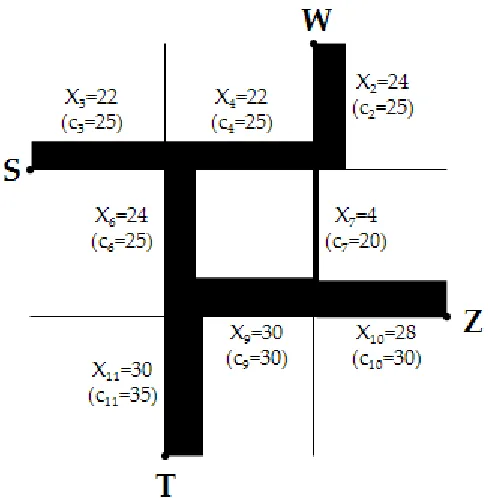
Framework of the traffic distribution problem has been elaborated based on linear programming approach, related to the following example. The transport network has been considered as follows in Fig. 1, where the possible origin zones were S and T, while the possible destination zones were W and Z.
Fig. 1.
Even in case of our simplified network, as well as in case of real transportation networks, there exist more alternative routes between OD zones. Routes were built up from graph edges (uj). Capacity of edges (cj) represented
the maximum possible number of travelers on a road in a given sample time period, travel time of the edges (tj) represented the time
needed to travel through the investigated infrastructure element. These parameters, as well as the transport demands (D) have been considered as constant, pre-defined data when determining the static system optimum of the problem. Road toll structure has been considered by the costs of travelling on the elements of the road network (kj was
the cost of travelling through edge j). The cost of travelling through i-th route (Ki)
was equal to the sum of the costs of the edges constructing the i-th route. Volumes of traffic on the routes (part-flows) have been estimated based on the road users’ willingness to pay for a route, which has been approximated by a linear function in our research.
The above introduced problem has been described as a linear programming problem. The variables of the model were the cost of the edges, which have been used to determine the part-flows of the alternative routes. Constraints have been derived from the capacity values of the edges and the travel demands appeared in a sample time period between OD pairs. The minimized objective function was the sum of products of the part-flows and travel time values of edges in a sample time period, while the most transport demands had to be satisfied.
When elaborating the framework of the optimization process, first step was the identification of possible alternative routes (Ui) in the investigated transportation
network, and the assignment of the part-flows (xi) among them, as presented below:
From zone S to W:
Alternative route: USW1: u3-u4-u2; part-flow
of route: x1
Alternative route: USW2: u3-u6-u9-u7-u2;
part-flow of route: x2
From zone S to Z:
Alternative route: USZ1: u3-u4-u7-u10; part-flow
of route: x3
Alternative route: USZ2: u3-u6-u9-u10; part-flow
of route: x4
From zone T to W:
Alternative route: UTW1: u11-u6-u4-u2;
part-flow of route: x5
Alternative route: UTW2: u11-u9-u7-u2; part-flow
of route: x6
From zone T to Z:
Alternative route: UTZ1: u11-u9-u10; part-flow
of route: x7
Alternative route: UTZ2: u11-u6-u4-u7-u10;
part-flow of route: x8
As part-flows of the routes depended on the cost of these routes, those travellers have also been considered, for who none of the free routes were appropriate based on the function of the willingness to pay. Transport demands of them have not been satisfied (they failed to travel because they were unwilling to pay the given costs). According to the system concept, the system could determine so “high” toll that it resulted missed travels if the capacity of the network (or any part of the network) was less than the emerging transport demands.
(with the same orientation as the real one) has been introduced for each real route as follows: U’SW1; U’SW2; U’SZ1; U’SZ2; U’TW1; U’TW2;
U’TZ1; U’TZ2. These fictive routes consisted
of fictive edges (u’1-u’12) with the same
orientation as the real edges.
In order to satisfy the most transport demands and avoid the use of fictive routes by the method when it was possible, extremely high travel time values for the edges of the fictive routes have been defined. Nevertheless, there was no need to constrain the capacity of the fictive edges. Part-flow of fictive routes have been indicated respectively by xi, i=9...16, while
traffic volume of the fictive edges have been indicated respectively by X’j, j=1...12. In the
framework of the solution, part-flows of the fictive routes have also been considered as variables, and have been taken into account when elaborating constraining conditions and the objective function. Note, that part-flows of the real routes were depending on the cost of the routes (willingness to pay function: xi(Ki), i=1...8).
Based on the considerations above, the following constraints have been introduced, as part of the framework of the solution process.
Values of xi have been required to be a
non-negative integer (as it represents traffic volumes of edges), as defined in Eq. 1.
(1)
Values of the cost of the edges have been required to be non-negative, as defined in Eq. 2.
(2)
Since travel demands between OD zones have been considered as pre-defined constant data, boundary conditions related to the traffic volume of the routes have been constructed according to Eq. 3-6., as travel demands between the OD zones have been distributed among the real and fictive routes between the corresponding zones.
(3)
(4)
(5)
(6)
In case of a linear optimization problem, constraining conditions, as well as the objective function have to be expressed in terms of the optimized variables. Hence, a 12x8 sized coefficient matrix (A) has been constructed with its elements (aij) to describe
This matrix made it possible to express the costs and traffic volumes of the routes based on the costs and traffic volumes of the edges. An arbitrary line of the matrix determined which routes contained the given edge (focusing on a line of the matrix: the value of a matrix component was 0 if the given edge was not part of the route described by the investigated column) and in accordance with this an arbitrary column of the matrix determined which edges were part of the given route (focusing on a column of the matrix: the value of a matrix component was 0 if the given route did not contain the edge described by the investigated line).
Cost of the real routes have been described in terms of the optimized variables according to Eq. 7, as part-flows of real routes were depending on the cost of the routes, based on the users’ willingness to pay, estimated by a linear function in our research.
(7)
Thus, when applying the elaborated framework, part-flows of the real routes can be expressed in terms of the optimized variables (cost of the edges) based on Eq. 7 and the willingness to pay function (xi(Ki),
i=1...8) defined by the example.
In the next step constraining inequalities derived from the pre-defined capacity constraints of real edges have been elaborated, as follows in Eq. 8. Traffic volume of the edges have been indicated by Xj, j=1...12.
(8)
Finally, the objective function has been defined. The aim was to minimize the total travel time of the vehicles go through the network in an investigated sample time period by varying the cost of the edges, and satisfying the most transport demands. Therefore, the objective function have been defined as the sum of products of total traffic and constant travel time of the real and fictive edges of the graph, as indicated in Eq. 9.
(9)
As part-flows of the fictive routes have also been involved in variables based on the introduced considerations, and have been taken into account in the objective function by using the traffic volume of the edges, we described the correspondences between traffic volumes of fictive routes and fictive edges in Eq. 10.
(10)
Therefore, framework of the optimization process has been elaborated by introducing equations 1-10, considering the constraining and boundary conditions as well as the objective function with linear formulas, based on static conditions and assumptions.
3. Verification of the Elaborated Method
Table 1
Transport Demands of the Transportation System
W Z
S 10 12
T 15 16
Values of capacity limits and travel time values of the edges of the investigated network have been defined in Table 2. As mentioned previously, extremely high travel
time values for the fictive edges have been defined, while there was no need to constrain the capacity of these edges.
Table 2
Characteristics of the Edges of the Network
Edges (uj) Capacity (cj) Travel time (tj)
u1 20 3
u2 25 3
u3 25 3
u4 25 3
u5 30 3
u6 25 3
u7 20 3
u8 25 3
u9 30 3
u10 30 3
u11 35 3
u12 25 3
u’1- u’12 ∞ 300
The function describing the road users’ willingness to pay for a route (in terms of the cost of the routes) has been estimated by a linear function indicated in Eq. 11.
(11)
The optimization problem has been solved with the intlinprog module of MATLAB software, which made it possible to constrain the value of some variables to integers.
Based on the syntax of the coding scheme in MATLAB, the following input attributes had to be defined, beside the variables containing the pre-defined constant data:
• f: vector containing the coefficients of the objective function;
• intcon: vector containing the ordinal number of integer variables;
• Coeff: matrix containing coefficients of constraining inequalities;
• constr: vector containing constant components of constraining inequalities, considering that (Coeff*x≤ constr);
• Aeq: matrix containing coefficients of constraining equalities;
• beq: vector containing constant components of constraining equalities, considering that (Aeq*x=beq);
where x was the vector of optimized variables (x=[k1, k2, …,k12, x9, x10, …,x16] 20 element
vector in our example). Pre-defined constant data have been coded as follows: constant parameters of the function describing the willingness to pay have been stored in R =(-3) and P=40 attributes, A auxiliary matrix has been stored as A, transport demands have been defined in D vector, capacity constraints of real edges have been defined in b vector and travel times of the real and fictive edges have been defined in t vector.
In intcon attribute, ordinal numbers of variables x9…x16 have been defined as these
optimized variables have been constrained to be integer in the elaborated framework, while lb has been defined as a 20 element vector with only zeros, as all variables have been constrained to be greater than or equal to 0 (see Eq. 1 and Eq. 2).
The definition of Coeff, constr, Aeq, beq and f
attributes required the application of some
advanced conversions and transformations, as described in the following sections of the article.
3.1. Definition of Coeff and constr
Attributes
Coef f ic ient s a nd con s t a nt t ag s of constraining inequalities have been stored in Coeff matrix and constr vector. Considering the number of variables (20 optimized variables), the constraining 12 inequalities related to the capacity limit of real edges (see Eq. 8), and the 8 inequalities related to part-flows of real routes (see Eq. 1, where i=1…8)), the size of Coeff is 20x20, while constr is a 20 element column vector. Based on its structure,
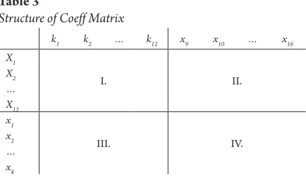
Coeff matrix can be divided to 4 quarters as indicated in Table 3. To define the elements of the matrix (coefficients related to variables), constraining inequalities have to be expressed in terms of the optimized variables.
Table 3
Structure of Coeff Matrix
k1 k2 … k12 x9 x10 … x16
X1
I. II.
X2 … X12 x1
III. IV.
x2 … x8
First two quarters of the matrix have been defined based on the constraining inequalities related to capacity constraints of the real edges, using Eq. 8 as a starting point. However, in Eq. 8, traffic volume of the edges have been expressed in terms of
(12)
After this conversion, traffic volumes of the edges have been expressed in terms of the optimized variables. Constant components then had to be rearranged from this expression to the right side of the inequalities and stored in constr vector. Furthermore, examining the coefficients related to P and
R*kj in case of Eq. 12 (consisting of only
the elements of A matrix), the following relationships can be observed: coefficients related to P are systematically the sum of rows of A matrix; coefficients related to R*kj
are systematically the linear combinations of the j-th row of A matrix with all rows of the matrix.
Applying these correspondences, and considering also that the necessary 12x12 linear combinations can be constructed by multiplying A matrix with its transposed matrix, the inequalities described by Eq. 12 have been written in a more clear form (Eq. 13), where the optimized variables have been multiplied out and therefore corresponding coefficients and constant tags can be easily defined for the coding scheme of MATLAB.
Related to n-th edge:
(13)
Based on these correspondences, elements of the first quarter of Coeff matrix have been defined as R*A*A’; elements of the second sextant of Coeff matrix were only zeros (as part-flows of fictive routes were not included in these inequalities), while the first 12 elements of constr vector have been defined as b-P*sum(A’) (note, that the capacity constraints have been stored in
b vector, while sum(A’) is the command in MATLAB to define a row-vector containing
the sum of columns of A matrix).
The third and fourth quarters of Coeff and the last 8 elements of constr have been defined based on the inequalities that describe that part-flows of real routes have to be non-negative, using Eq. 1 as starting point (considering i=1…8). Transformations have been applied again, as inequalities had to be expressed in terms of the optimized variables. Applying the introduced considerations of Eq. 11 and Eq. 7, the inequalities have been transformed as indicated in Eq. 14.
Related to i-th route:
(14)
After this conversion, part-flows of real edges have been expressed in terms of the optimized variables. Constant components (P in case of all inequalities here) then had to be rearranged from this expression to the right side of the inequalities and stored in constr vector. Examining the coefficients related to R*kj in case of Eq. 14 (consisting of
only the elements of A matrix), the following relationships can be observed: coefficients related to R*kj are systematically the sum of
the elements of the corresponding column of A matrix. Furthermore, it is necessary to multiply throughout the inequalities by (-1) as the relationship between Coeff and constr
is in the form of Coeff*x ≤ constr.
Applying the above considerations Eq. 14 can be written in a more clear form (Eq. 15), from which the corresponding coefficients and constant tags can be easily defined for the coding scheme of MATLAB.
Related to i-th route:
Based on these correspondences, elements of the third quarter of Coeff matrix have been defined as -R*A’; elements of the fourth sextant of Coeff matrix were only zeros (as part-flows of fictive routes were not included in these inequalities), while the last 8 elements of constr
vector were all equal to P.
3.2. Definition of Aeq and beq Attributes
Coef f ic ient s a nd con s t a nt t ag s of constraining equalities have been stored
in Aeq 4x20 matrix and beq 4 element column-vector, which have been defined based on the distribution of transport demands on the real and fictive edges, using Equations 3-6 as a starting point. In case of these equations, transformations had to be applied as part-f lows of real routes had to be expressed in terms of the optimized variables. Applying the introduced considerations of Eq. 11 and Eq. 7, equalities have been converted according to Eq. 15-18.
(15)
(16)
(17)
(18)
After this conversion, traffic volumes of the real edges have been expressed in terms of the optimized variables (cost of edges), while traffic volume of fictive routes were included in the optimized variables. Constant components then had to be rearranged from this expression to the right side of the equalities and stored in beq vector. Furthermore, examining the coefficients related to R*kj in case of Eq.
15-16 (consisting of only the elements of
A matrix), the following relationships can be observed: coefficients related to R*kj are
systematically the sum of those elements of A matrix, which are assigned by the j-th
row and the first two columns of the matrix in case of Eq. 15, the j-th row and the third and fourth columns of the matrix in case of Eq. 16, the j-th row and the fifth and sixth columns of the matrix in case of Eq. 17, and the j-th row and the last two columns of the matrix in case of Eq. 18.
Applying the above considerations, the constraining equalities have been defined in a more clear form (Eq. 19-22), where the optimized variables have been multiplied out and therefore corresponding coefficients and constant tags can be easily defined for the coding scheme of MATLAB.
(19)
(21)
(22)
Based on these correspondences, elements of Aeq matrix have been defined. The first row of it has been introduced in the article as an example: Aeq(1,1:12)=R*(A(1:12,1)’ +A(1:12,2)’); Aeq(1,13:20)=[1,1,0,0,0,0,0,0]. Besides that, the elements of beq vector have been defined as D-2*P.
3.3. Definition of f Vector Representing
the Coefficients of the Objective Function
Coefficients of the objective function have been stored in f 20 element vector. To define the elements of this vector, the objective function also had to be expressed in terms of the optimized variables, using Eq. 9 as a starting point, which contained the travel time values and traffic volumes of fictive and real edges. Traffic volumes of the real edges have already been expressed in terms of the optimized variables when determining
Coeff matrix, (see the left side of Eq. 12). The vector containing the traffic volumes of fictive edges can be constructed by multiplying A matrix by a vector containing the part-flows of fictive routes as follows in Eq. 23, since A matrix describes the correspondences between routes and edges.
(23)
Using these correspondences, the following elements have been used to define f vector in the coding scheme of MATLAB: t 24 element row-vector containing the travel time values of real and fictive edges; first 12 rows of Coeff matrix describing the coefficients of the traffic volume of real edges (without the constant components
that have been rearranged into constr vector, but these components have no effect on the optimal value of the variables, just on the value of the objective function); and the elements of A matrix which are exactly the coefficients related to the variables x9…
x16 in the expression describing the traffic
volume of fictive edges (see Eq. 23, and note that cost of the edges were not included in Eq. 23, therefore the coefficients related to them were 0). To be able to construct f
20 element vector, t 24 element row vector have been multiplied by V 24*20 element matrix, where V have been constructed as follows: first 12 row of V is the same as in
Coeff, while the last 12 row of V have been constructed by zero values in case of the first 12 column (related to kj variables) and
by A matrix in the last 8 columns (related to xi, i=9…16 variables), based on the above
mentioned considerations. Thus f vector have been defined as f=t*V.
3.3. Results of the Optimization Example
Based on the introduced considerations and transformations, optimized values of the variables have been calculated by the
intlinprog command of MATLAB as follows:
k2= 0 , 3 3 3 3 ; k3= 0 , 6 6 6 7 ; k4= 9 ;
k6= 0, 3333; k7=3, 6 6 67; k9= 8, 3333;
k1=k5=k8=k1 0=k1 1=k1 2= 0 ; x1 4= 1 ;
x9=x10=x11=x12=x13=x15= x16=0.
this F vector with V matrix (coefficients of the objective function), and then adding back the constant components that have been previously rearranged from the left side in Eq. 13. Thus, value of the objective function was 1752.
Based on our results, maximum load level of the system has been reached with the above introduced costs of edges, while only one transport demand remained unfulfilled. Thus, one traveler doesn’t want to pay
the defined cost of the route based on the function describing the willingness to pay. The missed travel has been loaded onto a fictive route (x14) between T and W zones.
Based on the constructed optimal road toll structure, part-flows of the alternative routes have been distributed as illustrated in Fig 2. Calculation of part-flows has been based on the function of willingness to pay applying the optimal cost values of the edges.
Fig. 2.
Sankey Diagram of the Optimal Traffic Distribution
As it can be seen in the Sankey diagram of the network, theoretically, the missed travel between T and W zones could have been loaded onto UTW1 as capacities of
the corresponding edges have not been exhausted. However, considering that the
constraining equalities of the model related to the transport demands would not be satisfied. In case of an autonomous transportation system this would mean that there are travelers whose transport demands have not been considered in case of the defined sample time period, but because of a current low costs of an alternative route they decide to start a journey, which would of course increase the load level of the system.
However, these considerations can serve as a basis for developing services for travelers in case of a dynamically changing road toll structure (e.g. an application that notifies travelers who would like to travel somewhere but their travel is not urgent so they could wait for cheaper costs).
The above mentioned phenomenon can be handled by defining the pre-defined transport demands as upper bounds of the willingness to pay function, since part-flows of the routes were calculated in terms of the costs based on that function. Although, the function of willingness to pay has been described by a simple linear function in case of the presented research, to consider the whole problem in a linear programming approach.
3. Conclusion
The research process has been implemented in two phases. In the first step a simplified transport system has been modeled where traffic volumes has been applied as basic system variable. In the second step road toll has been involved in the system as the basic variable supplemented by traffic volumes loaded to fictive edges (defined as fictive part flow) as additional variables. Transport demands and characteristics of the
infrastructure network have been considered as pre-defined static parameters, volume of traffic flows have been estimated depending on the road toll structure (considering the users’ willingness to pay, estimated by linear function).
The aim of the considered traffic distribution problem was to define the minimum of total travel time depending on total traffic appeared on the network in a sample time period of the model. The investigated transportation system and its elements were assumed to be fully autonomous in order to assign trip distribution tasks and users’ decision processes under the control of the system, providing the necessary requirements to achieve system optimum.
In the presented article, linear framework of the problem has been elaborated based on linear programming approach. The method has been verified by applying it on a simplified example. Based on the results, optimal road toll structure has been constructed by the algorithm satisfying the most transport demands and distributing the traffic to minimize the load level of the transport system. Optimal solution has been illustrated by a Sankey diagram.
References
Ansari, S.; Başdere, M.; Li, X.; Ouyang, Y.; Smilowitz, K. 2017. Advancements in continuous approximation models for logistics and transportation systems: 1996– 2016, Transportation Research Part B: Methodological 107: 229-252. DOI: https://doi.org/10.1016/j.trb.2017.09.019
Apronti, D.; Ksaibati, K.; Gerow, K.; Hepner, J.J. 2016. Estimating traffic volume on Wyoming low volume roads using linear and logistic regression methods,
Journal of Traffic and Transportation Engineering (English
Edition) 3(6): 493-506. DOI: https://doi.org/10.1016/j.
jtte.2016.02.004
Cavone, G.; Dotoli M.; Epicoco, N.; Seatzu, C. 2017. A decision making procedure for robust train rescheduling based on mixed integer linear programming and Data Envelopment Analysis, Applied Mathematical
Modelling 52: 255-273. DOI: https://doi.org/10.1016/j.
apm.2017.07.030
Hu, T.C.; Kahng, A.B. 2016. Linear and Integer
Programming Made Easy. Springer International
Publishing, Switzerland. 141 p. DOI: 10.1007/978-3-319-24001-5
Kumar, P.; Rosenberger, J.M.; Iqbal G.M.D. 2016. Mixed integer linear programming approaches for land use planning that limit urban sprawl, Computers & Industrial
Engineering 102: 33-43. DOI: https://doi.org/10.1016/j.
cie.2016.10.007
Kurczveil, T.; Becker, I.U. 2016. Optimization of novel charging infrastructures using linear programming,
IFAC-PapersOnLine 49(3): 227-230. DOI: https://doi.
org/10.1016/j.ifacol.2016.07.038
Ma, J.; Li, X.; Zhou, F.; Hao, W. 2017. Designing optimal autonomous vehicle sharing and reservation systems: A linear programming approach, Transportation Research
Part C: Emerging Technologies 84: 124-141. DOI: https://
doi.org/10.1016/j.trc.2017.08.022
Ma, W.; Qian, Z.S. 2017. On the variance of recurrent traffic f low for statistical traffic assignment,
Transportation Research Part C: Emerging Technologies 81:
57-82. DOI: https://doi.org/10.1016/j.trc.2017.05.009
Pauer, G.; Török, Á. 2017. Static system optimum of linear traffic distribution problem assuming an intelligent and autonomous transportation system (under publication), Periodica Polytechnica Transportation
Engineering.
Přibyl, O.; Svítek, M. 2015. System-oriented Approach to Smart Cities. In Proceedings of the 1st IEEE International
Smart Cities Conference, Guadalajara, Mexico, 1-8. DOI:
10.1109/ISC2.2015.7428760
Ryu, S.; Chen, A.; Choi, K. 2017. Solving the combined modal split and traffic assignment problem with two types of transit impedance function, European Journal
of Operational Research 257(3): 870-880. DOI: https://
doi.org/10.1016/j.ejor.2016.08.019
Yakimov, M. 2017. Optimal Models used to Provide Urban Transport Systems Efficiency and Safety,
Transportation Research Procedia 20: 702-708. DOI:
https://doi.org/10.1016/j.trpro.2017.01.114
Yang X.S. 2016. Engineering Mathematics with Examples
and Applications. Academic Press, 400 p. ISBN: