MULTIBODY DYNAMIC ANALYSIS
AND SIMULATION OF ENGINE
MODEL
Dr. S.C. Jaiswal
Department of Mechanical Engineering
Madan Mohan Malviya Engineering College, Gorakhpur, 273010, India E-mail: [email protected]
Tel: +91- 9839626792
Rahul Singh*
PG Student, Department of Mechanical Engineering
Madan Mohan Malviya Engineering College, Gorakhpur, 273010, India *Corresponding author; E-mail: [email protected]
Tel: +91-9839176917
Abstract
An assembly model for the internal combustion engine model has been proposed. The basis for the model is a study of earlier designs. The proposed design will run at a different speed, so the designers want to analyse the components, and in particular the stress in the connecting-rod, at the new speed.
The designer's question is: at what speed can the engine be run without the stress in the connecting rod exceeding the permissible stress for the material?
Keywords: Multibody Dynamic Simulation, Finite Element Analysis, HyperWorks, Engine Model
Introduction
In the last years finite element analysis has evolved as a powerful tool for supporting engineers in various fields of product development and research with the continuous increasing computational capabilities .These technique become more and more important for the effective development of competitive products.
IC (Internal Combustion) engines have been around for more than a century now and do not seem to be replaceable – not by any means completely - in the foreseeable future. The four-stroke variety is more commonly used as the source of motive power for applications such as automobiles. The performance of such an engine in terms of power, emissions and cost has changed drastically, from the time it was invented, though the basic governing thermodynamic cycle remains more or less the same. The four-stroke IC engine needs constant refinement as emission targets, which a vehicle must meet, become increasingly challenging. In addition, there is an ever-increasing demand on efficiency for which the need may be to step-up power-to-weight ratio of an engine as much as possible. Automotive companies bear huge cost in honing and updating IC engine technologies to meet some of the challenges mentioned. The advancement in computational techniques has greatly contributed to these efforts by offering opportunities for multiple design options to be evaluated virtually there by saving a great deal of investments associated with building of multiple prototypes.
analysis of an engine is the complex interactions between the domains mentioned. Consequently, at present, only simplified and semi-empirical tools based on lumped parameter modelling are available for modelling the multi-disciplinary behaviour of an IC engine system. With the advancement in CAE tools, it becomes easy to improve computational efficiency and to check practicability of design optimization.
The simulation methodology studied here is based on explicit dynamic finite element analysis using a commercial code in which contacts between relevant parts transferring motion are accounted for in the analysis. Crankshaft is a large component with a complex geometry in the engine, which converts the reciprocating displacement of the piston to a rotary motion with a four link mechanism. This study was conducted on a single cylinder four stroke cycle engine. Rotation output of an engine is a practical and applicable input to other devices since the linear displacement of an engine is not a smooth output as the displacement is caused by the combustion of gas in the combustion chamber. A crankshaft changes these sudden displacements to a smooth rotary output which is the input to many devices such as generators, pumps, compressors, etc.
This problem involves more than just an "FEA for stress analysis". In many situations, forces and restraints are not supplied. The designer has to estimate these and then perform the stress-analysis. This subject shows how to use OptiStruct / Analysis to integrate these two tasks. The components move as a mechanism - they make up a 4 bar mechanism with four joints.
Table: 1
Bar No. Bar Name
1 2 3 4
Crankshaft Connecting Rod
Piston
Table: 2
Joints Between Elements Motion
Crankshaft and Block Crankshaft and Connecting Rod
Connecting Rod and Piston Piston and Cylinder
Revolution Revolution Revolution Translation
So the first task is to calculate the forces in the components as the engine reciprocates. These forces should then be used to calculate the dynamic stresses in the component of interest - the connecting rod.
It is important that one realizes that the first task involves a rigid-body analysis, while the second involves a flexible-body analysis. The approach taken in this project makes use of the capability of OptiStruct / Analysis to mix both forms of analysis using component-mode synthesis.
The project explores the use of "bodies" and "joints" together with "elements" that the FE analyst is more familiar with.
Background
The project spans two separate branches of mechanics: continuum mechanics for stress analysis, and rigid body dynamics for calculation of forces.
The latter does not require 3D geometry, since the mass and inertial properties are adequate. However the availability of the 3D geometry makes it much easier to understand the results of the analysis. In addition, the use of the component mode synthesis approach means that the "flexibility" as calculated by the finite element method can be used to calculate dynamic stresses easily.
To appreciate the convenience of the method, it is interesting to contrast it with a "traditional" analysis. This would require that
the properties be calculated using a 3D model, typically a CAD model
these properties be transferred to a motion-simulation tool that can perform "dynamic" analysis, not simple "kinematic" analysis
the dynamic simulation be carried out and forces obtained as output
forces be transferred to a Finite Element model
the stress analysis be performed using the Finite Element model
With the integrated approach, the various "transfers" of data are eliminated, not only making the process easier and faster but also reducing scope for error.
Not only can forces be output and graphed, the stresses can be calculated automatically and displayed on the animation of the components
Planning and Organization
Most FE models contain a lot of data. There is the geometry (usually received from CAD) and the elements, restraints and loads. There is also some data that cannot be depicted graphically, such as the Modulus of Elasticity.
Planning how to organize this data goes a long way towards making the model easy to use.
The geometric entities (lines, surfaces, solids, points) are of no relevance to the FE solver. They are important only to help define the elements. The elements themselves, however, inherit some properties from the collector they are in - most important for us is the material data. We will ensure that the elements are in a collector that has been assigned the correct material.
We can also neglect some details in the geometry. This phase is called Geometry Clean-up. We will use this for convenience, rather than to control CPU-time and accuracy, since our focus is on setting up the multi-body problem, not on generating a high-quality mesh.
To sum up, our model will contain
one material collector
several collectors for elements
several collectors for solution-control
There may be other collectors which are not important for the FE solution. They will be used for convenience as and when required.
Multi-Body-Dynamics (MBD) Modelling
The modelling focus is on creation of joints and bodies.
OptiStruct / Analysis require that the two grids be used to define revolute and translational joints - one grid on each of the bodies. The grids that define the joints need to be on the axis of rotation, for a revolute joint. Since there may not be elements at the desired location, we make liberal use of "rigid" elements. These are equations that tell the solver that all "slave" nodes must move exactly as the "master" does. This approach allows us to define the grids for the joints at locations that are correct from the point of view of the multi-body solver.
Also, to ease visualization, we choose to create the joints with the grids in physically different locations. This way we can see the joint-definitions clearly. Once we have completed defining the joints, we move the grids and the associated bodies so that the "coincident grids" requirement is satisfied.
Loads and Restraints
This step is different from that of a "usual" Finite Element Analysis.
The use of "ground" bodies means we do not need any restraints on the FEA model. That is, we do not need any SPCs. Since this is a dynamic analysis, we will provide an initial velocity to the piston, to simulate the effect of a "kick-start".
Further, we define the interval for which we want to solve the problem. Note that unlike an FEA solution, the time-integration scheme used by the MBD solver embedded in OptiStruct / Analysis calculates the step-size for time-integration internally. Here, we specify the time-steps at which we want results reported.
This data is all that is required to generate the results.
Running OptiStruct/Analysis
Remember that the CPU time for analysis is an important criterion in any FEA. For a model that is finer than the one shown in the example, you may want to increase the RAM used. The on-line documentation explains how to do this.
Result and Analysis
The multi-body dynamic analysis of the engine is carried out on the computer equipped with 3GB RAM and an
Intel Core 2 duo processor for approximately hour of engine running.
Displacement
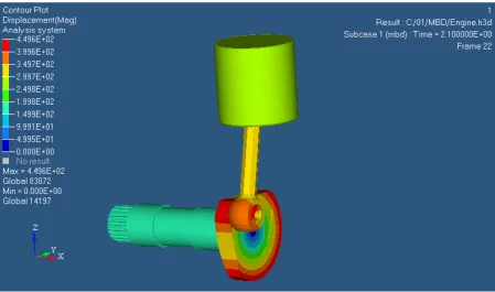
The contour plot of displacement shows displacement of various element of the model engine from their initial
positions. The red colour is used for showing maximum displacement while blue portion shows minimum
displacement. The maximum displacement comes out to be 4.496x102 mm and minimum displacement is zero
i.e. the centre axis of the crankshaft. The maximum displacement occurs in the crank and lower part of the
connecting rod.
Figure 2: Contour plot of displacement. Stress
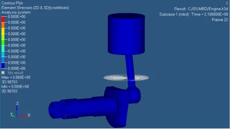
Dynamic analysis of the engine model results in more realistic stresses whereas static analysis provides
overestimated results.
The stresses in the engine components are generated due to inertia and the combustion of the fuel. These two
load sources cause both bending and torsional load on the crankshaft, bending on connecting rod, compressive
load on piston, etc. the initial starter velocity to the piston is given 4mm/s and it is seen that after this starter
velocity the engine starts running and the stress comes out to be zero. It means that this the starter velocity at
which engine runs is stress free. Beyond this velocity if engine runs, the stresses will be generated in the engine
Output files
The various output files are generated after running the analysis.
engine_frames.html
HTML report of the analysis, giving a
summary of the problem formulation and the
results from the final iteration.
engine.out
RADIOSS output file containing specific
information on the file set up, estimates for
the amount of RAM and disk space required
for the run, and compute time information.
Review this file for warnings and errors.
engine.h3d Binary
results file (Nodal results).
engine.stat
Summary of analysis process, providing CPU
information for each step during analysis
process.
engine _mbd.abf
Binary plotting file.
engine _mbd.h3d
Binary results file (Modal results).
engine
_mbd.log
Log file from OS-Motion containing the
information on the joints and markers,
simulation etc., which are specific to MBD
analysis.
engine _mbd.mrf
Binary results file for plotting.
engine
_mbd.xml
Model file in .xml format – solver
intermediate input deck.
Animations of motion are the classic output from a simple kinematic analysis. The first use of such an animation is simple a visual evaluation of motion for the designer to see if it is what is desired. More
sophisticated animations can be created to show motion from critical angles or even looking inside of parts,
which gives simulation a definite edge over building and running a physical prototype.
View the Results in HyperView
The results are viewed in HyperView module of HyperWorks which is launched from within the RADIOSS
panel of HyperMesh.
HyperView is a complete post-processing and visualization environment for finite element analysis (FEA),
multi-body system simulation, video and engineering data. The contour plot for displacement of engine
components from their initial position and stresses in several elements are easily viewed. The engine.h3d file
which is a binary result file (nodal result), is used for viewing the results. This file is fine to use because the .h3d
format contains both model and result.
Conclusions
This project investigated design and FE analysis of engine critical components from the base design of in house
exiting engine. The cost advantage of exiting proven design is used instead of going for a new development
process. First of all the critical parts are digitized by 3D modelling software. Stress analysis was performed
based on the input from proposed engine performance data, which comprised power output, crank, piston
assembly.
The boundary condition of connecting rod and crankshaft are applied over the respective FE models which was
created by using hyper mesh and the processing part was done by OptiStruct.
The result was viewed on HyperView. The contour plot for stress and displacement was plotted. The different
input velocities were taken at trial and error method. The contour plot for stress shows that there is no stress
developed in any component of the engine at a particular given speed of 4mm/s. So the model is successful for
that speed or less. Beyond this the stresses will develop and the model will fail.
In case of cylinder block, the pre-processing part was finished and the boundary conditions are identified, the FE
analysis part will be carried out later. The FE result is interpreted with the yield strength of thee component
material and FOS was calculated. The outcome of this analysis predicts the safer working of the parts under the
stated operating condition.
ACKNOWLEDGEMENT
I want to thanks Dr. Satya Pal Singh, (Asst. Professor, Applied Science Department, M.M.M. Engineering
College, Gorakhpur and also my family and friends Manish & Navneet for great support and help.
References
[3] AMBRÓSIO, J. and PEREIRA, M.S., 2003, “Desenvolvimentos Recentes no Cálculo Automático de Sistemas Mecânicos: Teoria a Aplicação”, Proceedings of VI Congresso Ibero-Americano de Engenharia Mecânica – CIBEM6, Departamento de Engenharia Mecânica, Universidade de Coimbra, Coimbra, edited by A.M. Dias, Volume I, pp. 1-20.
[4] ALSHAER, B.J., and LANKARANI, H.M., 2001, “Formulation of Dynamic Loads Generated By Lubricated Journal Bearings”,
Proceedings of DETC’01, ASME 2001 Design Engineering Technical Conferences and Computers and Information in Engineering Conference, Pittsburg, Pennsylvania, September 9-12, 8p.
[5] AMBRÓSIO, J.A.C., and GONÇALVES, J.P.C., 2001, “Vehicle crashworthiness design and analysis by means of nonlinear flexible multibody dynamics”, International Journal of Vehicle Design, 26(4), pp. 309-330.
[6] AMBRÓSIO, J., 2000, “Rigid and Flexible Multibody Dynamics Tools for the Simulation of Systems Subjected to Contact and Impact Conditions”, European Journal of Solids A/Solids, 19, pp. S23-44.
[7] HAUG, E.J., 1989, Computer-Aided Kinematics and Dynamics of Mechanical Systems - Volume I: Basic Methods, Allyn and Bacon, Boston, Massachusetts.
[8] HAUG, E.J., WEHAGE, R.A., and BARMAN, N.C., 1982, “Dynamic Analysis and Design of Constrained Mechanical Systems”,
Journal of Mechanical Design, 104, pp. 778-784.
[9] NIKRAVESH P.E., 1988, Computer-Aided Analysis of Mechanical Systems, Prentice Hall, Englewood Cliffs, New Jersey.
[10] SHABANA, A.A., 1997, “Flexible Multibody Dynamics: Review of Past and Recent Developments”, Multibody System Dynamics, 1, pp. 189-222.
[11] SHABANA, A.A., 1989, Dynamics of Multibody Systems, John Wiley and Sons, New York, New York.
[12] Moaveni, Saeed.,(2003). Finite Elements Analysis Theory and Application with Analysis, Pearson Education, Inc. 2nd Edition. p.6. [13] Reddy, J.N., (1993). An Introduction to the Finite Elements Method, Mc Graw Hill. 2nd Edition. p.5.
[14] Courant, R. (1943). Variational methods for the solution of problems of equilibrium and vibrations. Bull. Amer. Math. Soc. 49 123. [15] Hall, Allen S., Jr., Holowenko, Alfred R., Laughlin Herman G. (1961). Schaum’s Outline of Theory and Problems of Machine Design.
Schaum Publishing Co. p.-147.