Simulated Annealing based Optimization Model
for the Gossamer Protocol
Rama N.
#, Suganya R.
*#Department of Computer Science, Presidency College,
Chennai 600 005, India
*Department of Computer Science, Meenakshi College for Women, Chennai 600 024, India
and Research Scholar, Mother Teresa Women’s University, Kodaikanal 624 101, India
E-mail:[email protected]
Abstract
The use of low cost passive RFID tags has become very prevalent. Lightweight cryptography has evolved to address the security issues in these tags. The Gossamer protocol is a lightweight mutual authentication protocol which has guaranteed considerable security in these passive tags. As power is a major constraint in these tags, a detailed analysis of the power consumed by the Gossamer protocol was undertaken and results presented. It was determined that optimizing the power consumed by the protocol can result in substantial power savings and hence significantly enhance the performance of the RFID system. This paper proposes a new optimization model based on the simulated annealing method, that ensures the bounding of the number of power-crunching operations carried out in each run of the Gossamer protocol. The validity of the model is also established by the presentation and discussion of an experimental instance.
Keywords: Gossamer; RFID; Mutual Authentication Protocol; Optimization; Simulated Annealing.
1.
Introduction
Radio Frequency Identification (RFID) systems have become all but ubiquitous. Yet, the severely resource-constrained nature of the components of RFID systems places several constraints on the usage of these systems [1].
The main components of an RFID system are the RFID reader and RFID tags. An RFID tag is attached to any item that needs to be tracked or monitored. The RFID reader queries the tags from time to time and keeps track of them.
RFID tags are broadly classified as passive and active tags. Passive tags do not have even their own power source, and it is the RFID reader’s responsibility and prerogative to initiate the conversation. The tag draws power from the signal sent by the reader. Memory size and processing capability too are very limited in passive tags [2].
Mutual authentication is a crucial requirement that needs to be addressed in the case of RFID systems, for most applications of such systems involves the identification of the right tag by an authorized reader. Lightweight and yet secure mutual authentication protocols, therefore, become all-important. Ari Juels proposed the scheme of minimalist cryptography for this purpose [4]. This scheme is used for authentication between the reader and the tag through the exchange of messages. Inspired by this scheme, a family of Ultra-lightweight mutual authentication protocols was proposed by Pedro Peris Lopez et al [5, 6, 7, 8], of which the Gossamer protocol is a part [9].
The suitability of the Gossamer protocol for Class 1 RFID tags (passive tags) in terms of security, number of message exchanges needed for the authentication process and the memory demanded by the protocol, has been thoroughly studied. The performance of the protocol in terms of the amount of power involved in the generation of the messages was also analyzed by the authors [10].
The impact of the power consumed on the performance of RFID systems can never be over-emphasized. The lesser the power needed by the protocol the better will be the performance. As the RFID tag is drawing its power from the reader and the reader needs to energize multiple tags simultaneously, the lesser the power consumed by a single tag, the higher the number of tags the reader will be able to energize in one go. Thus, protocols proposed for mutual authentication between tag and reader as well as between tag pairs (such as those proposed by the authors [10]) will benefit to a large extent if the number of tags that can be read simultaneously by the reader increases. Optimization of the power consumed by the protocol provides a way to achieve this benefit.
This paper presents an optimization model for the Gossamer protocol, based on the Simulated Annealing optimization model. The Gossamer protocol extensively uses left-shift operations. It has been found during this study that restricting the number of shift operations (shift count) to within a specific range, directly contributes to power savings. The shift operations of a particular run of the protocol is determined by the input parameters n1 and n2, random numbers generated afresh by the
reader for each run of the protocol.
The model proposed in this work ensures that the random numbers generated contribute to a shift count that is bounded by desired upper and lower bound values. This fixing of a range for the shift count necessarily results in power savings, and hence contributes to enhanced performance of the RFID system as a whole. However, the model props up no boundaries on the values of the random numbers themselves, thereby posing no threat to the security of the system.
2.
Overview of Gossamer Protocol
The Gossamer Protocol is a lightweight mutual authentication protocol designed based on the minimalist cryptographic scheme. This section gives an overview of the protocol.
The basic assumptions of this protocol are as follows:
• Each RFID tag has a unique identification number (ID) that is 96 bits long.
• Each tag has the capability to store an IDS (Index pseudonym) and two keys k1 and k2, all
ofwhich are updated after each run of the protocol.
• The RFID reader has access to a database that has the values of ID, k1 and k2, indexed
through IDS for all tags in the RFID system’s scope.
• The communication channel between the reader and the database is secure and only trusted readers can have access to the database.
• The reader has a Pseudo Random Number Generator (PRNG) which generates two random numbers of at most 96 bits length for each run of the protocol.
The following is the list of operations and the notations used:
• Concatenation represented by ||
• XOR represented by ⊕
• Addition modulo 2m represented by +
• ROT(X,Y) defined as circular left shift of X by the value (Y mod 96)
a simple function called MixBits() is used to new random numbers using the random numbers
generated by the reader. This is a lightweight function having its base in genetic algorithms.
The protocol has the following phases (i) Tag Identification (ii) Mutual Authentication and (iii) Index pseudonym and key updating phase. In the tag identification phase, the reader sends a “hello” signal and the tag answers back with its IDS value. On receiving the IDS value, the reader uses it to index into the database and retrieves the corresponding ID and the keys k1 and k2. This marks the end
of tag identification phase.
Next, in the mutual authentication phase, first the reader is authenticated by the tag. This process is started off by the reader generating two random numbers n1 and n2, used extensively thereafter in
that particular round of the protocol. The values n1 and n2 are encrypted into two messages A and B,
which are concatenated with a third message C that reveals the identity of the reader to the tag, and sent to the tag. On receiving the message from the reader, the tag extracts the random numbers n1 and n2 from messages A and B respectively, and uses them to itself calculate C, which it then compares with the message C received from the reader. Thus, the tag authenticates the reader. Now the tag generates a message D in which it encrypts the ID and sends it to the reader, which the reader can verify. The reader thus authenticates the tag.
The IDS and keys k1 and k2 are updated after each run of the protocol both at the reader and the
tag ends. The updating of these values happens following the mutual authentication phase. The value of IDS, k1 and k2 of the last run of the protocol is also stored to handle synchronization problems. The
equations involved in generating the messages and updating the IDS and key values are given below: Mutual Authentication Phase:
Let n1 and n2 be the two random numbers generated.
, (1)
: , (2)
A ROT ROT IDS , , (3)
B ROT ROT IDS , , (4)
: ROT ROT , , (5)
: ROT ROT , , (6)
C ROT ROT , , (7)
D ROT ROT ID , , (8)
IDS and Key Updating Phase:
: MixBits , (9)
IDS ROT ROT IDS , , (10)
ROT ROT , , (11)
ROT ROT IDS , IDS , (12)
where c = 0x3243F6A8885A308D313198A2 (taken from π)
3.
Need for Optimization
The ROT() functional unit of the Gossamer protocol plays a very important role in determining the power consumed by the protocol. This is because this functional unit involves finding modulo 96, which requires repeated division, a highly demanding operation. Furthermore, repeated left-shifting is done, which also places a substantial demand on power. Over and above this, the fact is that the protocol applies this costly function twice while generating messages A, B, C and D and during each of the updates in the last phase of the protocol.
A single shift operation involves as many as 1000 gate transitions. Thus optimizing the number of shift operations (shift count) will save many thousands of gate transitions. This will in turn result in a great savings in the power consumed.
The number of shift operations to generate the messages varies depending on the values of the random numbers generated during each run of the protocol. A detailed analysis of this shift count range, done by varying the values of the random numbers n1 and n2 in different ranges, revealed that a
desired shift count range can be fixed and values of n1 and n2 can thus be chosen to produce shift
requirements for the protocol without compromising on the security, for the values of the random numbers can still be kept unbounded.
4.
The Proposed Optimization Model
4.1. Applying the Simulated Annealing Optimization Model
The optimization model proposed in this paper is based on Simulated Annealing [12], a classical optimization model for stochastic processes.
In the proposed model, a desired shift count range is identified, based on which an optimal space for the mean of the n1 values and mean of the n2 values is identified. The PRNG employed in the
reader can be designed to generate random numbers n1 and n2 in such a way that the mean of their
distributions falls within this optimal solution space, thus guaranteeing that the shift count lies within the desired range.
Since the Gossamer protocol uses the ROT() functional unit in many of its message-generation or value-updating algorithms, any one of these algorithms may be chosen to perform the aforesaid shift-count optimization. In this study, the message D has been chosen for the purpose, for it is this message that is generated by the resource-constrained tag.
The steps involved in identifying the optimal design space for the PRNG are as follows: 1. Fix the desired shift count range.
2. Generate a sample set of size 500 whose shift count range lies within the desired range. 3. Generate sets of size 500, of random number pairs n1 and n2.
4. Calculate the corresponding number of shifts involved (in message D in this case) for the generated sets.
5. Determine the correlation coefficient of the shift counts of the actual and desired sets of values.
6. Determine if the set is optimal or not by applying simulated annealing, the classical algorithm for which is given below.
Algorithm SIM {
S := Initial solution S0; T := Initial temperature T0;
while (stopping criterion is not satisfied) do {
while (not yet in equilibrium) do {
S’ := Some random neighbouring solution of S;
ΔE:= C(S’) - C(S); P := min(1, e-ΔE/KT);
q = random(0, 1); //a random number between 0 and 1
if q < P then
{
S := S’;
} }
Update T;
}
Output best solution; }
Temperature T depends on the system parameters that need to be optimized. In the present
the shift count range. The optimized system parameters as well as the solution space will therefore be expressed as distributions. In the present case, the SIM algorithm helps to generate the optimal distribution space for the mean values of n1 and n2 in order to minimize the shift count of the ROT()
functional unit.
4.2. The Experimental Setup
This section presents an experimental instance implemented to optimize the shift count range for the generation of message D. The process followed is detailed below:
1. 150 sets with 500 distinct pairs of n1 and n2 were generated. (The values of n1 and n2 are
unbounded in these sets. The values can also be bounded depending on the specific need of the application.)
2. The corresponding shift count value, λ, was calculated for each pair. λmax, λmin and λmean,
respectively the maximum, minimum and mean values of λ were determined for each of the 150 sets of values. Then, the overall mean values, viz. mean(λmax), mean(λmin) and
mean(λmean) were determined.
3. Based on these three values, three different desired shift count ranges, R1, R2 and R3 were
chosen in order to study the behaviour of the optimization model. They are o R1 : λmin = 40, λmax =100
o R2 : λmin = 20, λmax =150 o R3 : λmin = 10, λmax =170
4. For each desired range, one set with 500 distinct pairs of n1 and n2 that would produce a shift
count within the desired range were generated.
5. The Pearson’s correlation coefficient rA giving the measure of correlation between the
desired and actual shift counts was calculated. Now each of the 150 generated sets is represented by a triplet (m1, m2, rA) where m1 = mean(n1) and m2 = mean(n2). This triplet set
forms the input to the SIM algorithm.
6. A desired correlation coefficient value rD was fixed, and the optimization model was used to
determine whether the set under consideration would yield an optimal result. It is important to note that the optimization model makes a decision about the optimality of the set based not only on the correlation coefficient, but also on the values of n1 and n2.
7. The following are the definitions of the parameters of the SIM algorithm for the experimental setup.
• ΔE = rD - rA
• K = Boltzmann’s Constant = 1.3806503E-23
• T = ((1.0) * m1 + (0.8) * m2 ) * 1012
8.
The result was analyzed graphically to identify an optimal range for m1 and m2 such that anydistributions for n1 and n2 having their mean values in this range, would result in a shift count
that is within the desired range.
5.
Results, Graphical Analysis and Discussion
This section presents the results of the experimental setup detailed in Section 4. The input data set and the results of the application of the proposed optimization model are presented. Based on the output of the optimization, the data of 150 sets of values (m1, m2, rA) were thus split into two sets -
optimal and non-optimal – for each of the ranges R1, R2 and R3 considering two values for rD,
0.999999999999 and 0.988888888888.
3-Dimensional curves were fitted on the optimal and non-optimal data sets identified for R1, R2
and R3 for each of the considered rD values (Figures 1-6). The parameters for the graphs are m1 (
correlation coefficient, but has been extended in Figure 5 only to clearly display the shape of the curve.) The different colours in the graphs depict areas with different correlation coefficients.
The graphs were studied to determine the optimal ranges of m1 and m2 for a desired range of
correlation coefficient values, i.e. for a desired colour range, the ultimate aim being to generate distributions whose m1 and m2 valuesare such that the shift count would lie within the desired range of
shift count values.
5.1. Input Data Sets
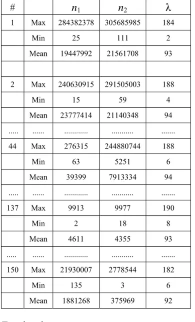
Table 1 gives the summary of the 150 input sets, each of which contains 500 sets of (n1, n2, λ).
The input sets are meant to be compared with a standard set of 500 values generated for each of the ranges R1, R2 and R3.
Table 1: Max, Min and Mean values of the input sets
# n1 n2 λ
1 Max 284382378 305685985 184
Min 25 111 2
Mean 19447992 21561708 93
2 Max 240630915 291505003 188
Min 15 59 4
Mean 23777414 21140348 94
... ... ... ... ...
44 Max 276315 244880744 188
Min 63 5251 6
Mean 39399 7913334 94
... ... ... ... ...
137 Max 9913 9977 190
Min 2 18 8
Mean 4611 4355 93
... ... ... ... ...
150 Max 21930007 2778544 182
Min 135 3 6
Mean 1881268 375969 92
For the above,
mean(λmax) = 185
mean(λmin) = 4
mean(λmean) = 91
The shift count ranges R1, R2 and R3 were chosen in such a way that λmax - λmin < mean(λmax) -
mean(λmin), and R1, R2 and R3 are in increasing order of λmax - λmin. Following are the results obtained
on comparing the 500 values of each of the 150 input data sets with a single standard data set generated for each of R1, R2 and R3.
5.2. R1: λmin = 40, λmax =100
Tables 2 and 3 show snapshots of the set of values generated for R1. Setting rD =
Table 2: Data Set for R1
# n1 n2 λ
1 4025 259821 48
2 74 1556 46
3 449 125901 90
4 211626 6753 96
... ... ... ...
496 303413 9521 100
497 20246 69417 69
498 206 1156 83
499 6343 151175 88
500 1236 1233 84
Table 3: Triplets (m1, m2, rA) for R1
# m1 m2 rA
1 19447992 21561708 0.985844303341463 2 23777414 21140348 0.978850765713698 3 25360551 22913238 0.986996885195985 4 21079821 23629477 0.989837520452073 ….. ……… …………. ……… 146 1605906 370644 0.983974430961630 147 1738372 377547 0.980081353343203 148 1773774 394059 0.978694550151069 149 1829292 401552 0.979856049496625 150 1881268 375969 0.984646942123398
Table 4: Optimal sets for rD = 0.999999999999
# m1 m2 rA
1 20300311 24105687 0.989053920957019
2 21907656 23446139 0.988131719871699
3 20029059 22216825 0.986801748019563
4 17438260 19823093 0.986800928857415
5 22385325 22801005 0.984896967632570
Table 5: Optimal Sets for rD = 0.988888888888
# m1 m2 rA
1 21748517 19429845 0.990574071159241
2 36266 8527681 0.990242985863639
3 21079821 23629477 0.989837520452073
... ... ... ... 25 21769342 22512452 0.982469164471311
26 21656794 22581737 0.981646517704330
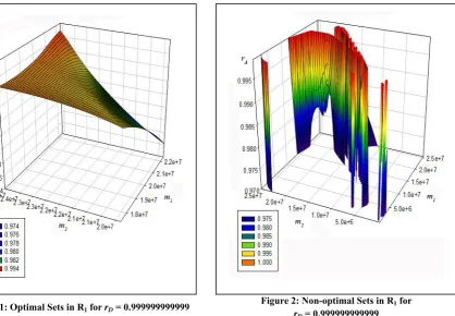
Figure 1 depicts the optimal region for R1 with rD = 0.999999999999, and Figure 2, the
non-optimal region for the same.
Figure 1: Optimal Sets in R1 for rD = 0.999999999999
Figure 2: Non-optimal Sets in R1 for
rD = 0.999999999999
In Figure 1,
• the dark green region represents optimal sets with
rA [0.982, 0.984] and m1, m2 [2.0*107, 2.2*107].
• the orange region represents optimal sets with
In Figure 2, however, the graph is a collection of vertical strands. In each strand the colour varies from blue to orange corresponding to rA [0.970, 0.999]. The implication of this is that the
distributions of random numbers n1 and n2 that have mean values m1 and m2in the range plotted, will not always result in distributions which have the desired shift count range. An instance from the graph is, when m1 [0, 5.0*106] and m2 [2.4*107, 2.5*107] the resulting distribution will not always be
optimal.
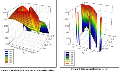
Figure 3 shows the optimal values of m1 and m2 with rD = 0.9888888888. Since the rD value has
been lowered, the number of data sets that are identified as optimal by the optimization model, naturally increases. This can also be gleaned from the area covered by the curve.
For instance, when m1 [5.0*106, 1.5*107] and m2 [2.0*107, 2.4*107], we get rA [0.995,
0.998] which means rA > rD. This is the orange region of the graph.
Figure 4, the representation of non-optimal values of m1 and m2 when rD = 0.9888888888, clearly
shows that for the plotted values, the shift count distribution will not always be optimal.
Figure 3: Optimal Sets in R1 for rD = 0.988888888888
Figure 4: Non-optimal Sets in R1 for
rD = 0.988888888888
5.3. R2: λmin = 20, λmax =150
Tables 6 and 7 show snapshots of the set of values generated for R2. For rD = 0.999999999999,
the proposed optimization model identified only 26 optimal sets out of the given 150 sets (Table 8). For rD = 0.988888888888, the optimization model identified all 150 sets as optimal.
Table 6: Data Set for R2
# n1 n2 λ
1 11136 43418 58
2 119194 3472950 114
3 2238 24533 142
4 81446 531 75
... ... ... ...
496 124105 487 86
497 6682 32781 87
498 41787 20223972 126
499 6092 7872 66
500 73862 1751775 123
Table 7: Triplets (m1, m2, rA) for R2
# m1 m2 rA
Table 8: Optimal sets for rD = 0.999999999999
# m1 m2 rA
1 41330 6953692 0.998492238269985
2 21079821 23629477 0.998280018961295
3 21958317 21464575 0.998164043161518 ... ... ... ...
25 21980517 22194863 0.995433670587354
26 22070903 20457930 0.995103104627828
R2 is larger than R1 and maps more closely to the shift count range of the input sets. This
considerably increases the number of sets that qualify as optimal, whereby the permissible range of values for m1 and m2 becomes wider.
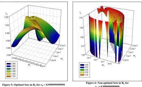
Figure 5 gives the graph depicting the optimal region for R2, where rD = 0.999999999999. Figure
6 represents the non-optimal regions for the same. In Figure 5
• the yellow region corresponds to the highest correlation and is obtained when
rA [1, 1], m1 [2.0*107, 2.5*107], m2 [2.0*107, 2.2*107].
• the bright blue region represents the lowest correlation and is obtained when
rA [0.985, 0.990], m1 [6.0*106, 1.0*107], m2 [2.0*107, 2.5*107].
Figure 5: Optimal Sets in R2 for rD = 0.999999999999
Figure 6: Non-optimal Sets in R2 for
rD = 0.999999999999
In Figure 4, we have rA [0.960, 1.000] and we have a jagged distribution. Thus, for instance,
for m1 [0, 5.0*106] and m2 [1.0*107, 1.0*107] the resulting distribution will not always yield shift
counts within the stipulated range.
Clearly, since all the input distributions considered have rA > 0.988888888888, when rD is set to
5.4. R3: λmin = 10, λmax =170
Tables 9 and 10 show snapshots of the set of values generated for R3. For rD = 0.999999999999
itself, the proposed optimization model identified all 150 sets as optimal.
Table 9: Data Set for R3
# n1 n2 λ
1 11544 158077 95
2 2440 250 134
3 14583 156910 119
4 77398 1544 88
... ... ... ...
496 176938 1123 101
497 918 47942 100
498 2354 1959 57
499 429 109767 114
500 304 1390 125
Table 10: Triplets (m1, m2, rA) for R3
# m1 m2 rA
1 19447992 21561708 0.997246073280999 2 23777414 21140348 0.996230884557808 3 25360551 22913238 0.997650264703144 4 21079821 23629477 0.998413071420934 … ………….. ………… ………. 146 1605906 370644 0.996325855732489 147 1738372 377547 0.996295473052837 148 1773774 394059 0.996061273070142 149 1829292 401552 0.996208183080908 150 1881268 375969 0.996726478973797
R3 is a closer approximation to the shift count range of the input sets, than R2. As a consequence
of this, all input sets were found to be optimal at both rD = 0.999999999999 and rD =
0.988888888888.
6.
Conclusion
The optimization model proposed in this paper is a new approach to achieving reduction in power consumed by fixing an optimal range for the number of shift operations performed in the Gossamer protocol.
Highlights of the optimization model proposed in this work are:
• The desired shift count range can be fixed depending on the security levels needed for the application.
• The equation for T can be fine-tuned to produce a larger or smaller design space.
• The design space for the PRNGs can be identified more precisely by generating a larger number of samples.
• The decision on how well the actual set needs to correlate with the desired set is left open to the designer.
• The model can also be applied to applications where the values of m1 and m2 are bounded.
Thus PRNGs can be designed to generate numbers with fixed word length which in turn reduces the hardware complexity and increases the processing speed at the reader end too.
The reduction in power consumption by the protocol results in improved performance of the RFID system. Since the parameters that are to be optimized are stochastic in nature, the Simulated Annealing method has been employed. The model has been detailed and its usage has also been demonstrated through examples. Detailed analysis of the graphical representations of the optimal sets and how it leads to fixing up the design space for PRNG is also presented.
Thus this model proves to be a successful optimization model that achieves significant reductions in the number of shift operations involved in the ROT functional unit of the Gossamer protocol. The beauty of this novel proposal is that such reduction is achieved without compromising on the security of the protocol, for the pseudo random numbers n1 and n2 are still left unbounded. Only the mean of these random numbers is restricted to fall within a standard distribution, causing the number of shift operations to become restricted to within certain boundaries.
References
[2] Class-1 Generation-2 UHF air interface protocol standard version 1.0.9: "Gen2", 2005, url: http://www.epcglobalinc.org/standards/ (last accessed on 10.01.2010).
[3] Denis Trcek and Pekka Jappinen. Non-Deterministic Lightweight Protocols for Security and Privacy in RFID Environments. RFID and Sensor Networks: Architectures, Protocols, Security and Integrations, Auerbach Publications, 2009.
[4] Ari Juels. Minimalist cryptography for low-cost RFID tags. Proceedings of SCN’04, vol. 3352 of LNCS, pages 149– 164, 2004.
[5] Pedro Peris-Lopez, J. C. Hernandez-Castro, J. M. Estevez-Tapiador, and A. Ribagorda. LMAP: A real lightweight mutual authentication protocol for low-cost RFID tags. Handbook of RFIDSec’06, 2006.
[6] Pedro Peris-Lopez, J. C. Hernandez-Castro, J. M. Estevez-Tapiador, and A. Ribagorda. M2AP: A minimalist mutual-authentication protocol for low-cost RFID tags. Proceedings of UIC’06, Vol. 4159 of LNCS, pages 912–923, 2006.
[7] Pedro Peris-Lopez, J. C. Hernandez-Castro, J. M. Estevez-Tapiador, and A. Ribagorda. EMAP: An efficient mutual authentication protocol for low-cost RFID tags. Proceedings of IS’06, Vol. 4277 of LNCS, pages 352–361, 2006.
[8] Chien H.Y., SASI. A New Ultralightweight RFID Authentication Protocol Providing Strong Authentication and Strong Integrity, IEEE Transactions on Dependable and Secure Computing, vol. 4(4), pp. 337–340. Oct.-Dec. 2007.
[9] Pedro Peris-Lopez, Julio Cesar Hernandez-Castro, Juan M. E. Tapiador, and Arturo Ribagorda. Advances in Ultralightweight Cryptography for Low-cost RFID Tags: Gossamer Protocol, Workshop on Information Security Applications, Vol. 5379 of LNCS, pages 56-68, 2008.
[10]Rama N. and Suganya R. Power Analysis of the Gossamer protocol for Passive RFID tags. Accepted for publication in International Journal of Wireless Communication and Networks March 2010.
[11]Rama N. and Suganya R. A Family of Gossamer-Based Mutual Authentication Protocols for Tag Pairs in RFID Systems. Reviewed and accepted for presentation and publication in the proceedings of ICMCS International Conference on Mathematics and Computer Science 2010, Loyola College, Chennai.