https://doi.org/10.5194/npg-25-375-2018 © Author(s) 2018. This work is distributed under the Creative Commons Attribution 4.0 License.
Time difference of arrival estimation of microseismic signals based
on alpha-stable distribution
Rui-Sheng Jia1,2, Yue Gong1,2, Yan-Jun Peng1,2, Hong-Mei Sun1,2, Xing-Li Zhang1,2, and Xin-Ming Lu1,2
1College of Computer Science and Engineering, Shandong University of Science and Technology, Qingdao 266590, China 2Shandong Province Key Laboratory of Wisdom Mine Information Technology, Shandong University of Science and Technology, Qingdao 266590, China
Correspondence:Rui-Sheng Jia ([email protected])
Received: 24 August 2017 – Discussion started: 27 September 2017
Revised: 25 April 2018 – Accepted: 25 April 2018 – Published: 14 May 2018
Abstract. Microseismic signals are generally considered to follow the Gauss distribution. A comparison of the dynamic characteristics of sample variance and the symmetry of mi-croseismic signals with the signals which followα-stable dis-tribution reveals that the microseismic signals have obvious pulse characteristics and that the probability density curve of the microseismic signal is approximately symmetric. Thus, the hypothesis that microseismic signals follow the symmet-ricα-stable distribution is proposed. On the premise of this hypothesis, the characteristic exponent α of the microseis-mic signals is obtained by utilizing the fractional low-order statistics, and then a new method of time difference of arrival (TDOA) estimation of microseismic signals based on frac-tional low-order covariance (FLOC) is proposed. Upon ap-plying this method to the TDOA estimation of Ricker wavelet simulation signals and real microseismic signals, experimen-tal results show that the FLOC method, which is based on the assumption of the symmetric α-stable distribution, leads to enhanced spatial resolution of the TDOA estimation relative to the generalized cross correlation (GCC) method, which is based on the assumption of the Gaussian distribution.
1 Introduction
Microseismic monitoring technology has been widely ap-plied to mine rock burst monitoring, oil and gas field frac-turing monitoring, reservoir seismic monitoring, slope sta-bility evaluation and so on. Seismic source location is one of the key technologies used (Zhao et al., 2017). The conven-tional seismic source localization method usually first needs
to pick up the P arrival time of multi-channel seismic signals and then calculate the time difference of arrival (TDOA) of the signals to solve the equation to obtain the source loca-tion (Schwarz et al., 2016). As a result, the accuracy of the calculated TDOA directly affects the accuracy of the seis-mic source location. However, in the process of actual oper-ation, the first arrival time of the microseismic signals is not obvious, and there is much external noise (Jia et al., 2015). Therefore, it becomes very difficult to determine the time dif-ference between waves from the same seismic source.
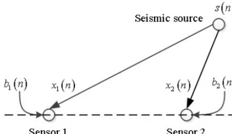
Figure 1.Two-sensor model of TDOA estimation.
Noisy microseismic signals have conspicuous non-stationary characteristics, such as impulsiveness and random-ness; therefore, they belong to the category of non-Gaussian signals. If the microseismic signal is simulated by Gaussian signal, it is inevitable that the TDOA algorithm will have se-rious performance degradation. To solve the problem in the-ory, we intend to introduce the α-stable distribution to de-scribe the microseismic signal and noise in the distribution model. Theα-stable distribution model has achieved excel-lence in the field of non-Gaussian signal processing, such as seismic inversion, speech de-noising and enhancement, sound source localization and mechanical fault diagnosis (Li and Yu, 2010; Yue et al., 2012; Zhang et al., 2014). However, its use is rare in research projects and publications on TDOA estimation of microseismic signals from the same seismic source. This paper intends to describe the characteristics of microseismic signals and noise with α-stable distributions, studies the impact of non-Gaussian noise on the spatial reso-lution of TDOA and proposes an improved TDOA algorithm based on fractional low-order covariance (FLOC). Compared with the traditional TDOA algorithm, this improved algo-rithm could inhibit both the Gaussian noise and theα-stable distribution noise.
2 The TDOA model
2.1 The basic model of TDOA
In order to facilitate data processing, the three component time travel curve of microseismic is first transformed into a set of energy gradient time travel curve (He et al., 2016). The basic model of TDOA is shown in Fig. 1. The original mi-croseismic signal is represented bys(n). It spreads to the two seismic geophonesS1andS2through the rock stratum. Due to different propagation paths, the time at which the signals arrive at the geophones are different.
If the microseismic acquisition system is discrete, the sig-nals received by the geophonesS1andS2can be expressed as
x1(n)=λ1s (n)+b1(n)
x2(n)=λ2s (n−D)+b2(n)
, (1)
In the above equation, s(n) represents the original signal.
Dis the time delay value.b1(n)andb2(n)are the external Gaussian noises. In addition,s(n),b1(n)andb2(n)are un-correlated.
Correlation analysis is commonly used to calculate the TDOA estimation of two signals. In the case that the sub-stance of the problem is not affected and the calculation is simplified, we takeλ1=λ2=1. Then, the cross correlation function of the two microseismic signalsx1(n)andx2(n)can be represented as
Rx1x2(τ )=E[x1(n) x2(n+τ )] (2)
=Rss(τ−D)+Rsb1(τ−D)+Rsb2(τ )+Rb1b2(τ ) ,
whereRss(·)represents the auto-correlation function of the original signal.Rpq(·)is the cross-correlation function of the two signalspandq. It is assumed thats(n),b1(n)andb2(n) are unrelated Gaussian noises. Then
Rsb1(τ−D)=Rsb2(τ )=Rb1b2(τ )=0. (3) Eq. (2) can be rewritten as
Rx1x2(τ )=Rss(τ−D) . (4)
The auto-correlation function has the property
|Rss(τ−D)| ≤Rss(0) . (5)
Therefore, Rss is maximized when τ−D=0. Thus, the TDOA estimation between the two seismic geophones can be expressed by the maximum ofRss(τ−D).
ˆ
D=argnmax τ
Rx1x2(τ−D)
o
2.2 The model ofα-stable distribution
In the process of microseismic monitoring, external noises are composed of man-made noises, mechanical vibration, etc. The common characteristics of these noises are that their time domain waveforms have conspicuous pulse character-istics, the energy diminishes from low to high frequencies and their corresponding probability density functions have a thicker tail than that of Gaussian signals. In the field of signal processing, this type of non-Gaussian noise is usually described by theα-stable distribution model.
Theα-stable distribution is a random signal model that can be applied to an extensive range of problems. Except for a few specific situations, there is no uniform probability den-sity function expression; therefore, Eq. (7) is used to express it (Shao and Nikias, 1993).
ϕ(m)=expjδm−γ|m|α1+jβsgn(m)ω (m, α) , (7)
ω (m, α)=
tanαπ
2 , α6=1
π
2log|m|, α=1
, (8)
sgn (m)=
1, m >0 0, m=0
−1, m <0
, (9)
where ϕ(m) is the characteristic function of the probabil-ity densprobabil-ity,αrepresents the characteristic exponent. Smaller values of αresult in thicker tails of the probability density function.βis the skew parameter, representing the deviation degree of signals. It is a symmetricα-stable distribution sig-nal when β=0, which is also called theSαS distribution.
γ is the scale parameter, representing the dispersion degree of signal around the location parameters, which is similar to the variance in the Gaussian distribution. δ is the location parameter, which is similar to the mean or mid-value in the Gaussian distribution.
We can infer from Eq. (7) that the corresponding eigen-function is the same as whenα=2. That is to say, the Gaus-sian distribution is a special case of the α-stable distribu-tion. When 0< α <2, Eq. (7) represents the eigenfunction of the signals following the non-Gaussian distribution, which is also called the fractional lower-orderα-stable distribution. 2.3 Non-Gaussian property of microseismic signals The difference in determining a signal between the Gaus-sian distribution and theα-stable distribution is that the lat-ter has stronger pulse characlat-teristics. Due to the existence of the pulse, the secondary moment of the observation data that follow the α-stable distribution is not convergent, and there is no limited high-order moment above the second or-der. However, the observation data that follow the Gaussian distribution have both stable secondary moment and limited high-order moment (Sun and Qiu, 2008). Therefore, whether or not the signal follows the Gaussian distribution can be
de-termined from whether or not the sample variance of the ob-served data is convergent.
If xi, i=1,2,3, . . .N represents the observed data se-quence and N represents the sample number of observed data. The dynamic sample variance of the firstk (1≤k≤N )
observed data is defined as
Sk2=1 k
k X
i=1
(xi−x, )2 (10)
x=1 k
k X
i=1
xi. (11)
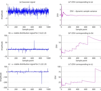
With the continuous increase ofk, ifSk2converges to a cer-tain value, the observed data sequence follows the Gaussian distribution. Otherwise, it follows theα-stable distribution. To illustrate the changes of the dynamic sample variance of the Gaussian signals and the α-stable distribution signals, three sets of random data are produced for comparison. The sample length of the three sets of data are all 1000 (Fig. 2), and Fig. 2a is a Gaussian signal. This means thatα=2.0,
β=0, γ=1,δ=0. Figure 2b is a random signal that fol-lows the α-stable distribution, and α=1.6, β=0, γ=1,
δ=0. Figure 2c is another random signal following theα -stable distribution, and α=1.2, β=0, γ=1, δ=0. The figures (Fig. 2d–e) are the dynamic sample variances corre-sponding to signals (Fig. 2a–c), respectively.
A comparison of the waveform characteristic of the sig-nals (Fig. 2a–c) shows that with the gradual decrease of the characteristic exponentα, the pulse characteristic of signals is enhanced. The signal (Fig. 2a) follows the Gaussian dis-tribution. Its pulse characteristic is not obvious, and its dy-namic sample variance converges to a stable value. The char-acteristic exponentα of the signal (Fig. 2b) is 1.6. It has a strong pulse characteristic. Its dynamic sample variance springs stepwise and does not converge to a stable value with an increase in sample points. The characteristic exponentα
of the signal (Fig. 2c) is 1.2. Its pulse characteristic is more obvious. The step amplitude of the dynamic sample variance increases sharply; therefore, it is more difficult to converge to a stable value.
We select a measured microseismic wave and calculate its dynamic sample variance according to Eq. (10) (Fig. 3). It shows that the microseismic signal’s dynamic sample vari-ance jumps stepwise and also does not converge to a sta-ble value. Thus, one can conclude that the microseismic sig-nal follows the fractiosig-nal lower-orderα-stable distribution. Through the analysis of a large number of seismic signals and the calculation of characteristic exponents, current liter-ature (Yue et al., 2013) shows that the characteristic exponent
0 200 400 600 800 1000 −10
−5 0
5 (a) Gaussian signal
Sample point
Amplitude
0 200 400 600 800 1000
0 1 2 3
4 (a*) DSV corresponding to (a)
Sample point
DSV
DSV − dynamic sample variance
0 200 400 600 800 1000
−50 0 50 100 (b)
α−stable distribution signal for (1.6,0,1,0)
Sample point
Amplitude
0 200 400 600 800 1000
0 5 10
15 (b*) DSV corresponding to (b)
Sample point
DSV
0 200 400 600 800 1000
−300 −200 −100 0 100 (c)
α−stable distribution signal for (1.2,0,1,0)
Sample point
Amplitude
0 200 400 600 800 1000
0 25 50 75
100 (c*) DSV corresponding to (c)
Sample point
DSV
Figure 2.Gaussian signal,α-stable distribution signal and their dynamic sample variance.
0 200 400 600 800 1000
−1.5 −1 −0.5 0 0.5 1
1.5x 10
−3 (a) Microseismic wave
Sample point
Amplitude
0 200 400 600 800 1000
0 0.2 0.4 0.6 0.8
1x 10
−7(b) DSV corresponding to (a)
Sample point
Dynamic sample variance
DSV − dynamic sample variance
−5 −4 −3 −2 −1 0 1 2 3 4 5 0
0.1 0.2 0.3 0.4 0.5
x
f(x
)
(a) α−stable densities,α = 0.7,γ= 1,δ= 0
β= 0.8
β= 0
β= −0.8
−300 −200 −1000 0 100 200 300
0.002 0.004 0.006 0.008 0.01 0.012
(b) α−stable densities of micro−seismic signals
x
f(x
)
Signal 1 Signal 2 Signal 3 Signal 4 Signal 5
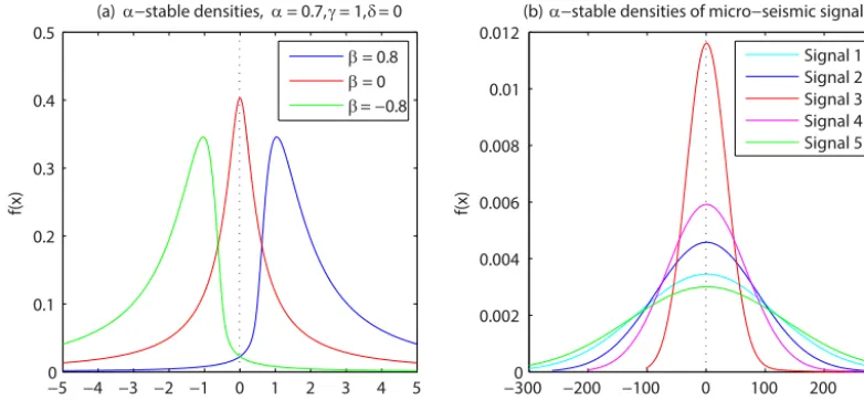
Figure 4. (a)Theα-stable densities with different skew parameter;(b)theα-stable densities of microseismic signals.
2.4 The determination of symmetry property of microseismic signal
Before the parameter estimation of theα-stable distribution, we should determine whether the distribution of the signal is symmetric. The methods for identifying symmetry are listed below:
1. Draw the probability density curve of the sample se-quence and observe the symmetry
2. Count the number of positive and negative values in the sample sequence. If the number of positive and negative values are approximately same, the signal is symmetric. Figure 4a shows that when the skew parameterβ=0, the probability density curve is symmetric; when β=0.8, the probability density curve is right-skewed; when β= −0.8, the probability density curve is left-skewed. Figure 4b shows five probability density curves of microseismic signals from the same seismic source. It is obvious that these curves are symmetric. As a result, the distribution of microseismic sig-nal is considered symmetric.
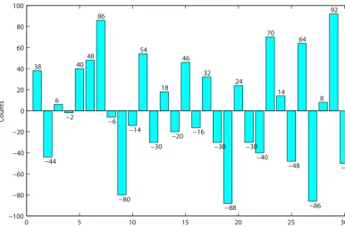
For further validation of the symmetry of microseismic signal, we randomly select 30 signals from the microseis-mic records in different places, truncate the continuous 3000 sampling points of each signal and then count the number of positive and negative values. The absolute value for the difference between the numbers of positive and negative is shown in Fig. 5.
According to the data in Fig. 5, we can use estimate max-imum likelihood estimator for parameters µ (difference of data number) and δ (standard error), and µ=1.8667 and
δ=26.8356 are obtained. Compared with the 3000 of sam-ple data, the microseismic signal is approximately consid-ered symmetric.
In conclusion, the microseismic signal follows the sym-metric α-stable distribution, which is also called the SαS
distribution. Because theα-stable distribution does not have limited secondary and high-order moment, the above TDOA method is based on the assumption that the secondary mo-ment (or high-order momo-ment) and the Gaussian noise shows serious performance degradation. It is necessary to do some research on the new TDOA algorithm based on the low-order statistics.
3 The improved TDOA estimation algorithm 3.1 The TDOA estimation based on FLOC
According to the study of Sect. 2.4, the microseismic signals and noises are more consistent with theα-stable distribution. Therefore, this paper is intended to describe the characteris-tics of microseismic signals and noises byα-stable distribu-tion. ON this basis, an improved TDOA algorithm based on fractional low-order covariance (FLOC) is proposed. Com-pared with the traditional TDOA algorithm, the improved algorithm has a good suppression effect on the noise ofα -stable distribution noise and Gauss noise.
In the case that the noise follows the α-stable distribu-tion, an existing study (Ma and Nikias, 1995) puts forward a TDOA algorithm based on fractional low-order covariance (FLOC). The FLOC of two signalsxi(t )(i=1,2) is defined as
Rd(τ )=E
h
x2(t )<A>x1(t+τ )<B>
i
, (12)
0≤A <α
2, 0≤B <
α
0 5 10 15 20 25 30 −100
−80 −60 −40 −20 0 20 40 60 80 100
38
−44 6
−2
4048
86
−6
−80 −14
54
−30 18
−20 46
−16 32
−30
−88 24
−30 −40
70
14
−48 64
−86 8
92
−50
Serial number of microseismic record
Count
s
Figure 5.The absolute value for the difference between the positive and negative counts in each microseismic record.
x<c>= |x|csgn(x) ,sgn(x)=
1, x >0 0, x=0
−1, x <0
, (13)
whereAandB represent the fractional low-order exponents of the two input signals xi(t ) (i=1,2), respectively. τ is the translation relative to the signal x1(t )when calculating FLOC. The TDOA estimation can be obtained by detecting the peak of the functionRd(τ ).
D= −argnmax τ [Rd(τ )]
o
(14) The FLOC algorithm can be used for the TDOA estimation of microseismic signals. If the two microseismic signal sam-ples arexi(n)(i=1,2;n=1,2, . . ., N ), Eq. (12) can be ex-pressed by
ˆ Rd(τ )=
1
N N X
n=1
|x2(n)|A|x1(n+τ )|B·sgn [x2(n)x1(n+τ )],
0≤A <α
2, 0≤B <
α
2, 0< α≤2. (15)
The TDOA estimation can be obtained by detecting the peak of the functionRˆd(τ ).
ˆ
D= −argnmax τ
h ˆ Rd(τ )
io
(16) The TDOA method based on FLOC requires very few calcu-lations and its real-time implementation is simple. However,
theαparameter needs to be estimated in advance; otherwise, the FLOC algorithm will have serious performance degra-dation and will lead to incorrect results whenAandB are greater thanα/2.
3.2 The estimation of the characteristic exponentα
For the random variableX, which follows theα-stable dis-tribution, the fractional lower-order moment is defined as
E |X|p, 0< p < α≤2.pis the order of fractional lower-order moment. From the Zolotarev theorem (Zolotarev, 1966) we obtain
E |X|p=C (p, α) γp/α, (17)
C (p, α)=
2p0p+210 1−p α
√
π 0 1−p
2
, (18)
whereαrepresents the characteristic exponent,γ represents the scale parameter and0(·)represents the gamma function. If the random variableX follows theSαS distribution, a study has found that there is a negative-order moment in the
SαS distribution (Ma and Nikias,1995). Equation (17) can then be changed to
E |X|p
=C (p, α) γp/α, −1< p < α≤2, (19) because
Eq. (20) is continuous at the pointp=0 after the introduc-tion of negative-order moment. IfY =log|X|,E epYis the moment-generating function ofY and
E
epY
= ∞ X
k=0
E
Yk pk
k! =C (p, α) γ
p/α. (21)
Then any order moments ofY are limited and
EYk= d k
dpk
C (p, α) γp/α p=0. (22)
This can be simplified to
E(Y )=Ce
1 α−1
+1
αlogγ , (23)
whereCe=0.57721566. . .is a Euler constant. Then
Var(Y )=En[Y−E(Y )]2o=π
2
6
1
α2+ 1 2
. (24)
For the microseismic signals Yi (i=1,2, . . ., N, N is the sampling number), and the mean and variance can be ob-tained by Eqs. (25) and (26), respectively.
Y = 1 N
N X
i=1
Yi (25)
Var(Y )= 1 N
N X
i=1
Yi−Y 2
(26)
Plugging in the value gained from Eq. (26) into Eq. (24), we can obtain an estimated value of α. Then, the value ofαis plugged into Eq. (23), and we obtain the value ofγ.
3.3 Algorithm procedures
If xi(n) (i=1,2;n=1,2, . . ., N) represents the sample of two microseismic signals from the same seismic source, the TDOA algorithm is shown below:
Step 1: for a given sequence of discrete signal x1(n) and
x2(n), calculate their characteristic exponentsα1andα2 according to Eqs. (24), (25) and (26);
Step 2: assigningA=0.95×α1
2 andB= 0.95×α2
2 to find that 0≤A <α1
2, 0≤B < α2
2, 0.95 is an empirical value; Step 3: add the Hanning window to x1(n) and x2(n),
and set the window lengths to max(size(x1(n))) and max(size(x2(n))). The cross-correlation functionRˆd(τ ) ofx1(n)andx2(n)is calculated according to Eq. (15); Step 4: detect the peak of the function Rˆd(τ ). Then, the
TDOA estimationDˆ can be obtained.
4 Simulation and analysis
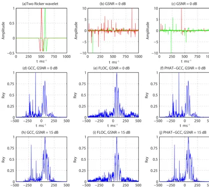
The signals Ricker1 and Ricker2 used in the simulation are two Ricker wavelets. Their spectral peak frequency is 25 Hz. The sampling frequency is 1 kHz, and the number of sam-pling points is 1000. The time delay between the two Ricker wavelets is set to 70 ms (Fig. 6a). The generalized signal-to-noise ratio (GSNR) is defined in Eq. (27) and used to describe the power ratio of signal and noise (Ma and Nikias, 1996). GSNR=10 lgσs
γ. (27)
In the equation,σsrepresents the signal power, andγ repre-sents the noise figure of theα-stable distribution.
4.1 Experiment 1
The spatial resolution on TDOA estimation of the general-ized cross correlation (GCC), PHAT-GCC (phase transfer– generalized correlation) method based on the Gaussian dis-tribution and the FLOC method based on the non-Gaussian distribution are compared and verified.α-stable distribution noises to the two Ricker wavelets are added. The parameter of theα-stable distribution (α,β,γ,δ) is set to (1.2, 0, 1, 0). Because of the randomness ofα-stable distribution noises, the two noises are independent of each other. The two Ricker wavelets with added noises are shown in Fig. 6b and c. In the case ofα-stable distribution noises, the TDOA estima-tion results of the GCC, PHAT-GCC method and the FLOC method when GSNR=0 dB and GSNR=15 dB are shown in Fig. 6d–j.
It is evident from Fig. 6d, f, h and j that the GCC and PHAT-GCC method shows serious performance degradation when GSNR=0 dB and GSNR=15 dB. There are several peak positions in the curve so that the correct result is dif-ficult to get. However, the FLOC method has a strong anti-interference ability. The peak appears at 70 ms and can esti-mate the time delay correctly.
4.2 Experiment 2
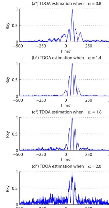
The influence of differentαto the TDOA estimation results are verified. The two noises are generated randomly when
αtakes different values between 0 and 2 and are added to Ricker1 and Ricker2, respectively. When GSNR=0 dB, the TDOA estimation result of the two signals with noises ob-tained by the FLOC method is shown in Fig. 7. Figure 7a–d show the waveforms of Ricker1 and Ricker2 with different noise signals added to these waveforms. Figure 7a∗–d∗show the corresponding TDOA estimation results.
0 250 500 750 1000 −0.5
0 0.5
1 (a)Two Ricker wavelet
Amplitude
0 250 500 750 1000
−10 −5 0 5
10 (b) GSNR = 0 dB
Amplitude
−500 −2500 0 250 500
0.25 0.5 0.75 1
Rxy
(d) GCC, GSNR = 0 dB
−500 −2500 0 250 500
0.25 0.5 0.75 1
Rxy
(e) FLOC, GSNR = 0 dB
−500 −2500 0 250 500
0.25 0.5 0.75 1
Rxy
(f) PHAT−GCC, GSNR = 0 dB
0 250 500 750 1000
−10 −5 0 5
10 (c) GSNR = 0 dB
t ms–1
Amplitude
−500 −2500 0 250 500
0.25 0.5 0.75 1
Rxy
(h) GCC, GSNR = 15 dB
−500 −2500 0 250 500
0.25 0.5 0.75 1
Rxy
(i) FLOC, GSNR = 15 dB
−500 −2500 0 250 500
0.25 0.5 0.75 1
Rxy
(j) PHAT−GCC, GSNR = 15 dB t ms–1
t ms–1
t ms–1
t ms–1
t ms–1 t ms–1
t ms–1 t ms–1
Figure 6.Comparison of the TDOA estimation results of GCC, FLOC and PHAT-GCC.
estimation result: 70 ms. Therefore, the FLOC method per-forms well irrespective of the noise and follows the Gaussian distribution or theα-stable distribution.
5 Case study
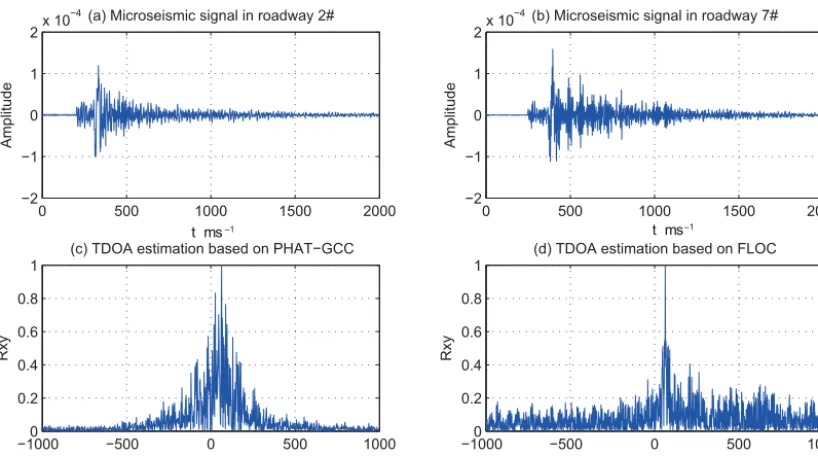
To verify the effectiveness of the FLOC method for TDOA estimation of real microseismic signals, we select eight mi-croseismic signals from the same seismic source to do the experiment. The eight signals come from the ISS microseis-mic monitoring system of a coal mine in central China. Seis-mic geophones are laid along the mining roadway every 50 m in the system. The frequency bandwidth of the seismic geo-phones is between 3 and 2000 Hz. The data acquisition fre-quency is 1 kHz. For convenience of comparing and analyz-ing the experiment results, the first 2000 samplanalyz-ing points of each waveform are picked as the data object. The P arrival time of each microseismic signal is recorded manually, and
the time delay between any two of the microseismic signals as a reference of the experimental result is calculated.
As an example, the microseismic signals in roadway nos. 2 and 7 are selected to explain the result. The waveforms of the microseismic signals after interception are shown in Fig. 8a and b. The time delay between the two signals obtained by manual method is 19 ms. First, when the microseismic signal follows the Gaussian distribution, the PHAT-GCC method, which, of the GCC methods, performs best, is chosen for the TDOA estimation of microseismic signals from the same seismic source. The result is shown in Fig. 8c. Second, when the microseismic signal follows the α-stable distribution, FLOC is used for the TDOA estimation. The characteristic exponentαof the two picked signals are calculated accord-ing to Eqs. (23), (24) and (25).α2=1.802,α7=1.835 are obtained as results. According to Step 2 in Sect. 3.3, assign
0 200 400 600 800 1000 −2
0 2 4
Amplitude
(a) α = 0.8
−5000 −250 0 250 500
0.5 1
Rxy
(a*) TDOA estimation when α= 0.8
0 200 400 600 800 1000 −2
0 2 4
Amplitude
(b) α= 1.4
−5000 −250 0 250 500
0.5 1
Rxy
(b*) TDOA estimation when α= 1.4
0 200 400 600 800 1000 −5
0 5
Amplitude
(c) α= 1.8
−5000 −250 0 250 500
0.5 1
Rxy
(c*) TDOA estimation when α= 1.8
0 200 400 600 800 1000 −5
0 5
Amplitude
(d) α= 2.0
−5000 −250 0 250 500
0.5 1
Rxy
(d*) TDOA estimation when α= 2.0 t ms–1
t ms–1
t ms–1
t ms–1 t ms–1
t ms–1 t ms–1
t ms–1
Figure 7.The influence of differentαto the TDOA estimation result.
Figure 8c and d show that the two methods both obtain the correct result, 19 ms, but the peak of the FLOC method is sharper than the GCC method. This implies that the FLOC method performs better.
Each of the eight microseismic signals is considered to be a set of data following the α-stable distribution. Their characteristic exponentαvalues are calculated according to Eqs. (23), (24) and (25) and are shown in the table (Table 1). The values are between 1.802 and 1.913 (Fig. 9). It can be seen that the characteristic exponent α values of all of the signals are less than 2. According to the data in Table 1, we can use estimate maximum likelihood estimator for parame-tersµ(difference of data number) andδ(standard error), and
µ=1.8550,δ=0.0377 can be obtained.
We can obtain 28 pairs of microseismic signals by the pair combination of the eight signals in Table 1. The comparison of TDOA estimations obtained by the PHAT-GCC, FLOC and manual method is shown in the table (Table 2).
An analysis of tables (Tables 1, 2) indicates that the pulse of actual microseismic signal is stronger than the one
fol-Table 1.The characteristic exponentαof microseismic signal.
Roadway Characteristic Roadway Characteristic
number exponentα number exponentα
1 1.864 5 1.913
2 1.802 6 1.857
3 1.822 7 1.835
4 1.901 8 1.846
Table 2.The comparison of TDOA estimation results of microseis-mic signal.
TDOA error=0 ms error≤3 ms error≤5 ms method percentage percentage percentage
FLOC 96.43 % 100 % 100 %
0 500 1000 1500 2000 −2
−1 0 1
2x 10
−4
Amplitude
(a) Microseismic signal in roadway 2#
0 500 1000 1500 2000
−2 −1 0 1
2x 10
−4
Amplitude
(b) Microseismic signal in roadway 7#
−10000 −500 0 500 1000
0.2 0.4 0.6 0.8 1
Rxy
(c) TDOA estimation based on PHAT−GCC
−10000 −500 0 500 1000
0.2 0.4 0.6 0.8 1
Rxy
(d) TDOA estimation based on FLOC
t ms–1
t ms–1
t ms–1
t ms–1
Figure 8.The comparison of TDOA estimation results based on PHAT-GCC and FLOC.
1# 2# 3# 4# 5# 6# 7# 8# 1.5
1.6 1.7 1.8 1.9 2
Roadway number
α
Figure 9.Comparison of the characteristic exponentαof eight mi-croseismic signals.
lowing the Gaussian distribution. Because the characteristic exponent of the actual microseismic signal is less than 2, it is considered to be a signal following theα-stable distribution. Based on this observation, we can say that the spatial res-olution of the FLOC method is better than the PHAT-GCC method at TDOA estimation of microseismic signals.
6 Conclusions
Through the analysis of the convergence of dynamic sam-ple variance, the microseismic signal with noises is shown to follow theα-stable distribution. The analysis of the sym-metry of probability density curve of the sample sequence proves that the microseismic signal is approximately sym-metric. Therefore, it is more reasonable to regard the micro-seismic signal with noises as theα-stable distribution signal.
Because of the absence of second-order statistics of α -stable distribution, one cannot obtain optimal or correct esti-mation values via the traditional TDOA method based on the Gaussian distribution.
Microseismic monitoring data obtained from a coal mine in central China are used for TDOA estimation based on the GCC method and the FLOC method to study cases when the microseismic signals follow the Gaussian distribution and the
α-stable distribution. In the comparison of the results and the time delay obtained manually, we observe that the FLOC method performs better than the traditional GCC method ir-respective of whether the noise follows the Gaussian distri-bution or theα-stable distribution. This method is suitable for the TDOA estimation of microseismic signals from the same seismic source.
Data availability. The microseismic data we use in this paper are
derived from a coal mine. These microseismic data are not pub-lished online and are not intended to be pubpub-lished, because these data contain technical secrets of the coal mine.
Competing interests. The authors declare that they have no conflict
of interest.
Acknowledgements. This work is funded by the State Key
Foundation (2015M582117), Qingdao Postdoctoral Applied Research Project and Special Project Fund of Taishan Scholars of Shandong Province.
Edited by: Shaun Lovejoy
Reviewed by: two anonymous referees
References
Carrier, A. and Got, J. L.: A maximum a posteriori probability time-delay estimation for seismic signals, Geophys. J. Int., 198, 1543– 1553, 2014.
Choudhuri, S., Bharadwaj, S., Roy, N., Ghosh, A., and Ali, S. S.: Tapering the sky response for angular power spectrum estima-tion from low-frequency radio-interferometric data, Mon. Not. R. Astron. Soc., 459, 151–156, 2016.
Cornelis, B., Doclo, S., Tim, V. D. B., Moonen, M., and Wouters, J.: Theoretical analysis of binaural multi-microphone noise re-duction techniques, IEEE T. Audio Speech, 18, 342–355, 2010. Gedalyahu, K. and Eldar, Y. C.: Time-delay estimation from
low-rate samples: a union of subspaces approach, IEEE T. Signal Pro-ces., 58, 3017–3031, 2010.
Harada, K.: Nonparametric spectral estimation of phase noise in modulated signals based on complementary autocorrelation, IEEE T. Signal Proces., 62, 4479–4489, 2014.
He, X. L., She, T. L., and Gao, F.: A new method for picking up arrival times of seismic p and s waves automatically, Chinese J. Geophys.-Ch., 59, 2519–2527, 2016.
Hertz, D. and Azaria, M.: Time delay estimation between two phase shifted signals via generalized cross-correlation methods, Signal Process., 8, 235–257, 1985.
Hinich, M. J. and Wilson, G. R.: Time delay estimation using the cross bispectrum, IEEE T. Signal Proces., 40, 106–113 1992. Hou, H., Sheng, G., Miao, P., Li, X., and Jiang, X.: Time-delay
es-timation algorithm of partial discharge UHF signals in substa-tion based on bispectrum, Proceedings of the Chinese Society for Electrical Engineering, 33, 208–214, 2013 (in Chinese with English abstract).
Jia, R.-S., Zhao, T.-B., Sun, H.-M., and Yan, X.-H.: Microseismic signal denoising method based on empirical mode decomposi-tion and Independent component analysis, Chinese J. Geophys.-Ch., 58, 1013–1023, https://doi.org/10.6038/cjg20150326, 2015. Jia, R.-S., Liang, Y. Q., Hua, Y. C., Sun, H. M., and Xia, F. F.: Suppressing non-stationary random noise in microseis-mic data by using ensemble empirical mode decomposition and permutation entropy, J. Appl. Geophys., 133, 132–140, https://doi.org/10.1016/j.jappgeo.2016.08.001, 2016.
Jin, Z., Jiang, M., Sui, Q., Sai, Y., Lu, S., Cao, Y., Zhang, F., and Jia, L.: Acoustic emission localization technique based on general-ized cross-correlation time difference estimation algorithm, Chi-nese J. Sensor. Actuat., 26, 1513–1518, 2013 (in ChiChi-nese with English abstract).
Kang, J. W., Whang, Y., Ko, B. H., and Kim, K. S.: Generalized cross-correlation properties of chu sequences, IEEE T. Inform. Theory, 58, 438–444, 2012.
Knapp, C. and Carter, G.: The generalized correlation method for estimation of time delay, IEEE T. Acoust. Speech, 24, 320–327, 1976.
Li, C. and Yu, G.: A new statistical model for rolling element bear-ing fault signals based on alpha-stable distribution, 2th Interna-tional Conference on Computer Modeling and Simulation, Sanya China, 22–24 January 2010, 4, 386–390, 2010.
Ma, X. and Nikias, C. L.: Parameter estimation and blind channel identification in impulsive signal environments, IEEE T. Signal Proces., 43, 2884–2897, 1995.
Ma, X. and Nikias, C. L.: Joint estimation of time delay and fre-quency delay in impulsive noise using fractional lower order statistics, EEE T. Signal Proces., 44, 2669–2687, 1996. Park, J., Shevlyakov, G., and Kim, K.: Maximin distributed
detec-tion in the presence of impulsive alpha-stable noise, IEEE T. Wirel. Commun., 10, 1687–1691, 2011.
Qiu, T. S., You, G. H., Sha, L., Zhao, X. P., and Gao, Y.: A phase spectrum time delay estimation method based on frequency dif-ference compensation, Journal of Dalian University of Technol-ogy, 52, 90–94, 2012 (in Chinese with English abstract). Salvati, D. and Canazza, S.: Adaptive time delay estimation
us-ing filter length constraints for source localization in reverberant acoustic environments, Signal Process. Lett., 20, 507–510, 2013. Schwarz, B., Bauer, A., and Gajewski, D.: Passive seismic source localization via common reflection surface attributes, Stud. Geo-phys. Geod., 60, 531–546, 2016.
Shao, M. and Nikias, C. L.: Signal processing with fractional lower order moments: stable processes and their applications, P. IEEE, 81, 987–1010, 1993.
Souden, M., Benesty, J., and Affes, S.: Broadband source localiza-tion from an eigen analysis perspective, IEEE T. Audio Speech, 18, 1575–1587, 2010.
Sun, H. M., Jia, R. S., Du, Q. Q., and Fu, Y.: Cross-correlation anal-ysis and time delay estimation of a homologous microseismic signal based on the Hilbert-Huang transform, Comput. Geosci., 91, 98–104, https://doi.org/10.1016/j.cageo.2016.03.012, 2016. Sun, Y. M. and Qiu, T. S.: The new HB weighted time delay
esti-mation algorithm under impulsive signal environments, J. Syst. Eng. Electron., 19, 1102–1108, 2008.
Wang, P., Zhang, X., Sun, G., Xu, L., and Xu, J.: Adap-tive time delay estimation algorithm for indoor near-field electromagnetic ranging, Int. J. Commun. Syst., 30, e3113, https://doi.org/10.1002/dac.3113, 2017.
Xu, N., Dai, F., Sha, C., Lei, Y., and Li, B.: Microseismic signal characterization and numerical simulation of concrete beam sub-jected to three-point bending fracture, J. Sensors, 10, 1–11, 2015. Youn, D. H., Ahmed, N., and Carter, G. C.: On using the LMS al-gorithm for time delay estimation, IEEE T. Acoust. Speech, 30, 798–801, 1982.
Yue, B., Peng, Z., and Zhang, Q.: Seismic inversion method with α-stable distribution, Chinese J. Geophys.-Ch., 55, 1307–1317, 2012 (in Chinese with English abstract).
Yue, B., Peng, Z., and Zhang, Q.:α-stable distribution seismic sig-nal characteristic exponent estimation, Joursig-nal of Jilin University (Earth science edition), 43, 2026–2034, 2013 (in Chinese with English abstract).
Zhang, D. W., Bao, C. C., and Xia, B. Y.: Source localization based on time delay estimation in complex environment, J. Commun., 35, 183–190, 2014.
acoustic computed tomography, Appl. Therm. Eng., 75, 958– 966, 2015.
Zhao, T. B., Guo, W. Y., Tan, Y. L., Lu, C. P., and Wang, C. W.: Case histories of rock bursts under complicated geological con-ditions, B. Eng. Geol. Environ., https://doi.org/10.1007/s10064-017-1014-7, online first, 2017.