https://doi.org/10.5194/amt-12-2979-2019 © Author(s) 2019. This work is distributed under the Creative Commons Attribution 4.0 License.
Use of polarimetric radar measurements to constrain simulated
convective cell evolution: a pilot study with Lagrangian tracking
Ann M. Fridlind1, Marcus van Lier-Walqui1,2, Scott Collis3, Scott E. Giangrande4, Robert C. Jackson3, Xiaowen Li5,6, Toshihisa Matsui6,7, Richard Orville8, Mark H. Picel4, Daniel Rosenfeld9, Alexander Ryzhkov10, Richard Weitz8, and Pengfei Zhang10,11
1NASA Goddard Institute for Space Studies, New York, NY, USA
2Center for Climate Systems Research, Columbia University, New York, NY, USA 3DOE Argonne National Laboratory, Argonne, IL, USA
4DOE Brookhaven National Laboratory, Upton, NY, USA
5Goddard Earth Science and Technology and Research, Morgan State University, Baltimore, MD, USA 6NASA Goddard Space Flight Center, Greenbelt, MD, USA
7Earth System Science Interdisciplinary Center, University of Maryland, College Park, MD, USA 8Department of Atmospheric Sciences, Texas A&M University, College Station, TX, USA
9The Fredy & Nadine Hermann Institute of Earth Studies, The Hebrew University of Jerusalem, Jerusalem, Israel 10Cooperative Institute for Mesoscale Meteorological Studies, National Weather Center, Norman, OK, USA 11NOAA/OAR National Severe Storms Laboratory, Norman, OK, USA
Correspondence:Ann M. Fridlind ([email protected]) Received: 21 December 2018 – Discussion started: 15 January 2019 Revised: 12 April 2019 – Accepted: 18 April 2019 – Published: 3 June 2019
Abstract.To probe the potential value of a radar-driven field campaign to constrain simulation of isolated convection sub-ject to a strong aerosol perturbation, convective cells ob-served by the operational KHGX weather radar in the vicin-ity of Houston, Texas, are examined individually and statis-tically. Cells observed in a single case study of onshore flow conditions during July 2013 are first examined and compared with cells in a regional model simulation. Observed and sim-ulated cells are objectively identified and tracked from ob-served or calculated positive specific differential phase (KDP)
above the melting level, which is related to the presence of supercooled liquid water. Several observed and simulated cells are subjectively selected for further examination. Below the melting level, we compare sequential cross sections of re-trieved and simulated raindrop size distribution parameters. Above the melting level, we examine time series ofKDPand
radar differential reflectivity (ZDR) statistics from
observa-tions and calculated from simulated supercooled rain proper-ties, alongside simulated vertical wind and supercooled rain mixing ratio statistics. Results indicate that the operational weather radar measurements offer multiple constraints on
the properties of simulated convective cells, with substantial value added from derivedKDPand retrieved rain properties.
been generally strengthened that aerosol pollution from an-thropogenic activities is likely to have commonly offset re-gional and global radiative forcing of the Earth’s climate by anthropogenic greenhouse gases to date, but uncertainty, especially in aerosol effects on cloud-related forcing, still remains high (IPCC, 2013). Although such anthropogenic aerosol radiative forcing will be diminutive relative to that from buildup of anthropogenic greenhouse gases on cen-tury timescales under most scenarios, the variable degree to which anthropogenic aerosols offset greenhouse gas warm-ing in simulations that reproduce the observational record of surface temperature change since preindustrial times con-tinues to be a leading factor limiting simulation constraints on Earth’s climate sensitivity (e.g., Kiehl, 2007). Fundamen-tal understanding of the relationships between global cloud processes and atmospheric circulations and thermodynam-ics is another leading factor, as demonstrated by studies that find grossly differing predicted climate sensitivities asso-ciated with differing parameterization of fundamental pro-cesses such as convective mixing, convective aggregation, or cloud glaciation (e.g., Sherwood et al., 2014; Mauritsen and Stevens, 2015; Tan et al., 2016).
Addressing aerosol–cloud–precipitation–climate interac-tions locally and regionally, Rosenfeld et al. (2014) describe how field campaigns designed to measure closed energy and moisture budgets over relatively large domains, referred to as box flux closure experiments, could help advance under-standing of primary microphysical mechanisms and regional-scale dynamical feedbacks. Here we further consider how ob-servations designed for a box flux closure experiment could be amended to aid attribution of primary cloud responses to aerosol variability, specifically in the case of convective cells responding to a boundary layer aerosol perturbation. The ob-servational objective of establishing microphysical and dy-namical differences across a population of evolving convec-tive cells is considered an amendment because observing the details of updraft cell evolution within a flux closure cam-paign box well poses a significant additional challenge be-yond constraining fluxes at the box boundaries. However, there may be overlapping utility in the use of polarimetric radar systems to observe convective cell spatial evolution within the box and to provide state-of-the-art retrievals of
tal formation (Pruppacher and Klett, 1997). For individual drops, that barrier would not be spontaneously overcome in commonly occurring dilute solution drops until they are su-percooled by at least 30◦C below their melting temperature
stronger updrafts, all else being equal. This is borne out in simulations under some environmental conditions to an ex-tent that may be dependent on the complexity of the micro-physics scheme, and has been supported by large-domain sta-tistical studies (e.g., Fan et al., 2013, and references therein). Conversely, it has also been repeatedly demonstrated that differing microphysics schemes predict grossly differing up-draft and cloud properties, at least in part owing to a lack of observational constraints on important factors such as liquid water content and ice properties, making it extremely chal-lenging to establish whether any scheme is performing sub-stantially better than any other for the correct reasons (e.g., Fridlind et al., 2012; Varble et al., 2014a, b; Wang et al., 2015).
Polarimetric radar systems such as those operated by the National Weather Service Next-Generation Radar (NEXRAD) program (NOAA, 2017) provide a rich source of information about the size distribution, phase, and shape of hydrometeors (Zrni´c and Ryzhkov, 1999), which is espe-cially valuable for the study of convective updraft physics be-cause of the paucity of such data available from aircraft (e.g., Loney et al., 2002; Fridlind et al., 2015; Snyder et al., 2015). Comparison of reflectivity and phase-shift differentials be-tween horizontal and vertical radar polarizations yields dif-ferential reflectivity (ZDR) and specific differential phase
(KDP), which are related to the presence of horizontally
aligned oblate or prolate hydrometeors when positive (Bringi and Chandrasekar, 2001). Vertically elongated columns of positiveZDR andKDPthat extend above the environmental
melting level (ZDRandKDPcolumns) have been generally
attributed to the presence of supercooled liquid associated with a deep convective updraft that is not otherwise identi-fiable from reflectivity alone (Bringi et al., 1996; Hubbert et al., 1998; Loney et al., 2002; Kumjian et al., 2014a). Re-cent studies suggest a strong connection between KDPand
ZDR columns and other metrics of deep convective
activ-ity such as overshooting tops (Homeyer and Kumjian, 2015) and lighting flash rate and updraft mass flux (van Lier-Walqui et al., 2016). Observations also show differences inKDP
ver-susZDRcolumn morphology (Zrni´c et al., 2001; Loney et al.,
2002; Kumjian and Ryzhkov, 2008), which have been at-tributed to differing sensitivities to hydrometeor size distri-bution and phase characteristics (e.g., Kumjian et al., 2014b; Snyder et al., 2017b). However, precise attribution of spe-cific morphological features at various wavelengths remains a challenge due to a paucity of colocated in situ measure-ments, the complexity of updraft microphysics, and uncer-tainties in calculating hydrometeor electromagnetic proper-ties, especially for mixed-phase particles (e.g., Loney et al., 2002; Ryzhkov et al., 2011; Snyder et al., 2013, 2017b).
Many past studies have effectively examined deep con-vective cells using observations from individual radar scans (e.g., Hubbert et al., 1998; Loney et al., 2002). Tracking con-vective cells or other identified features in time increases the amount of information that can be gleaned from scanning
radar because temporal aspects such as cell lifetime can be quantified (e.g., Stein et al., 2015). Feature identification and tracking have wide applications in the atmospheric sciences. Many studies have applied unsupervised feature identifica-tion to locating cloud regimes using satellite observaidentifica-tions (e.g., Jakob and Tselioudis, 2003; Rossow et al., 2005; Pope et al., 2009). Automatic tracking is perhaps most widely ap-plied in nowcasting using surface radar observations (Dixon and Wiener, 1993; Johnson et al., 1998; Scharenbroich et al., 2010; Limpert et el., 2015). Surface radar observations gen-erally have a frequency on the order of 5–10 min, and the rate of successful tracking can be 60 % to 90 % according to Lak-shmanan and Smith (2010). Here we investigate isolated con-vective cells, which have smaller sizes and shorter life spans than the storm features in most radar weather tracking. The KDPcolumn identification algorithm used in this pilot study
was described by van Lier-Walqui et al. (2016). We also in-troduce a more efficient tracking algorithm for compilation of long-term statistics using parallel computing.
For the study of updraft microphysics we target conditions where a relatively strong aerosol perturbation exists and up-drafts are not being strongly driven by synoptic flow, which are commonly satisfied in the vicinity of Houston when there is onshore flow. Such conditions increase the likelihood of observationally establishing the statistical relationship be-tween aerosol and updraft properties, which can in turn be used as a constraint for evaluating and improving models. The Houston region currently offers the significant advantage of a lightning mapping array (LMA; Orville et al., 2012), which can provide independent three-dimensional informa-tion on updraft locainforma-tion and phase (e.g., van Lier-Walqui et al., 2016). The objectives of this pilot study are to establish the lifetime and observable properties of typical isolated con-vective cells and to demonstrate comparison of isolated cell observations with an example regional model simulation.
Next in Sect. 2, we describe the data sources and methods of analyzing isolated cell features in a selected case study and in long-term statistics. Results are presented in Sect. 3. In Sect. 4, we discuss results in the context of pilot study objectives.
2 Methodology 2.1 Data sources
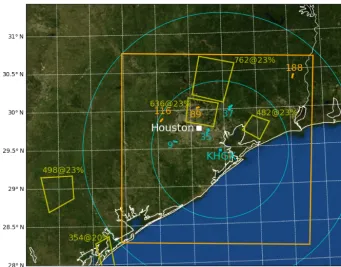
Figure 1.Map of Houston region (white symbol marks city center), NU-WRF inner domain boundaries (orange square), KHGX NEXRAD radar location (cyan symbol with 100 and 200 km range rings), tracks of three example features from KHGXKDPobservations (cyan tracks numbered 9, 35, and 37) and from NU-WRFqroutput (orange tracks numbered 89, 116, and 188), and CCN number concentration and supersaturation retrieved from satellite data (within yellow boxes in number per cubic centimeter and as a percentage, respectively).
which makes it inappropriate for estimating regions of de-creasing propagation phase shift (i.e., regions where differ-ential phase shift, orKDP, is negative). Conversely, this fact
makes the LP algorithm better suited for identifying regions of positiveKDP, such as those associated with oblate
parti-cles like rain and liquid-coated hail that are expected in con-vective updrafts.
From a NASA Unified Weather Research and Forecast-ing (NU-WRF; Peters-Lidard et al. , 2015) model simula-tion, 5 min frequency outputs were analyzed. The model is configured with a 600 km×600 km outer domain grid cen-tered around Houston with 3 km horizontal grid spacing and, centered within the outer domain, a nested 300 km×300 km inner domain with 120 vertical levels and 500 m horizontal grid spacing (Fig. 1). Time steps of 12 and 2 s were used on the outer and inner grids, respectively. The same physics op-tions were used on both grids. The planetary boundary layer parameterization used the Mellor–Yamada–Nakanishi–Niino level 2.5 turbulent kinetic energy scheme (Nakanishi and Ni-ino, 2009). The Morrison et al. (2009) two-moment cloud microphysics scheme was used with a fixed droplet number concentration of 100 cm−3, and reflectivity at horizontal po-larization (ZHH) was calculated using the resulting
hydrome-teor size distributions with temperature-dependent refractive indices following Blahak et al. (2011). The Goddard broad-band two-stream radiative transfer scheme was used to
cal-culate radiative fluxes and atmospheric heating rates (Chou and Suarez, 1999, 2001; Matsui et al., 2018a). Model terrain was smoothed from the 30 s and 0.9 km U.S. Geological Sur-vey topography data for both domains, and land cover was mapped from 30 s MODIS land use data. Sea surface tem-perature and atmospheric initial and lateral boundary condi-tions are obtained from 6-hourly output of the Modern-Era Retrospective Analysis for Research and Applications Ver-sion 2 (MERRA-2; Bosilovich et al., 2015). Land surface ini-tial conditions (soil moisture and temperature) were derived from a 6-month spin-up (Kumar et al., 2007) of the Noah land surface model (LSM) using the MERRA-Land mete-orological forcing (Reichle et al., 2011). The LSM spin-up was conducted at the grid configuration identical to that used in the simulation. The simulation was started at 00:00 UTC on 8 June 2013 and integrated for 24 h. At 16:00–17:00 UTC, convective cells begin to appear within 100 km of the KHGX radar location in both the simulation and the observations.
effec-tive radius with an estimated uncertainty of 30 % (Rosenfeld et al., 2016). Rain mass-weighted mean diameter (Dm; the
fourth moment of the drop number size distribution divided by the third moment) and generalized intercept parameter (Nw) (see Testud et al., 2001) were retrieved from KHGX
data at elevations below the melting level following Ryzhkov et al. (2014), with an estimated uncertainty of roughly 5 %– 10 % in Dm and log(Nw)(Thurai et al., 2012). Collocated
rain rate has been retrieved from the specific attenuationA using the R(A) methodology that is most efficient at the S band, with an estimated bias less than 6 % (Ryzhkov et al., 2014; Zhang et al., 2017). Lightning flashes were estimated from raw very-high frequency (VHF) signals detected by the LMA. A simple set of heuristics was used to cluster VHF sources into discrete flashes, similar to MacGorman et al. (2008): the first 10 VHF sources in a flash are required to be within 0.25 s and 3 km of one another, and each flash is not allowed to exceed 3 s in total duration and must be composed of at least 10 VHF sources.
For comparison with the additional observational data, we calculate several further quantities from standard NU-WRF outputs. From rain mixing ratio and number concentration, we use the microphysics scheme assumptions and limitations on rain size distribution properties to calculate rainDmand
Nw. FromDmwe further estimate rainZDRfollowing Bringi
and Chandrasekar (2001, their Eq. 7.14a). From bothDmand
Nw, rainKDPis estimated as described in Appendix A.
2.2 KDPcolumn tracking
Convective cells can be objectively identified and tracked using observed or forward-calculated radar variables (ZHH,
ZDR,KDP) or model variables such as rain water mixing
ra-tio (qr). From three-dimensional gridded KHGX data for this
study,KDP-based values were first calculated in each model
column following
ξ = zf
Z
zm
φ (z)(z−zm)dz, (1)
wherezmandzfare the melting and homogeneous freezing
heights andφ (z)is the value ofKDPin each column grid cell,
similar to the approach taken in van Lier-Walqui et al. (2016). Such a metric favors both theφ (z)value and its height. Since hydrometeor size distribution assumptions made in bulk mi-crophysics schemes such as that used in the NU-WRF sim-ulation are not generally adequate to forward simulate fully realistic KDPfields (e.g., Ryzhkov et al., 2011), analogous
values were calculated from NU-WRF output first using rain water mixing ratio (qr), and then using rain KDP estimated
as described in Appendix A. In observations, fixedzmandzf
grid cell bottom and top edge values of 4.5 and 9 km, respec-tively, were estimated from 00:00 and 12:00 Z soundings at Lake Charles, Louisiana, such that the lowest gridded radar volume was above 0◦C and the highest gridded radar volume
below−40◦C. Similar heights were found from soundings at Corpus Christi, Texas. In NU-WRF output, fixedzmandzf
values of 4.1 and 10 km were taken from the inner domain grid layer mean temperature profile. The conclusions of this pilot study are not sensitive to the precise choice ofzmandzf
values. However, we note that obtaining accurate time- and space-dependentzmandzfvalues from observations could be
challenging. It could conceivably be preferable to derive rele-vant integration limits from observed and forward-simulated radar variables in future work.
Using the two-dimensional fields of ξ values, features were identified and tracked using Trackpy, an open-source Python object tracking toolbox. Whether using observations or model data, regional relative maxima were identified and tracked using Trackpy’s predictive tracker with a maximum tracked object velocity of 30 m s−1and a “memory” of three frames to allow for splitting or merging cells to be followed. Paths with five or fewer time frames were discarded. We note that this procedure serves to objectively identify a “track-able” cell without requiring a definition of cell initiation.
When comparing observed and simulated reflectivity fields from tracked objects, the variables and tracking param-eters described above were subjectively deemed adequate for the purposes of this pilot study. A more in-depth future study would motivate additional focus on optimizing such choices for any specific conditions of interest. We also found that tracking performed onξ values obtained from simulatedqr
versus simulatedKDPdid not influence study results, likely
attributable to the fact that theKDPestimation approach used
here is so closely linked toqralone. In the following we
fo-cus only on simulated objects tracked fromξbased onKDP.
2.3 Long-term cell tracking, introducing TINT
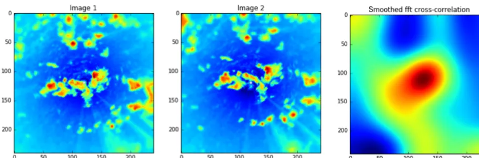
Figure 2.Two reflectivity factor snapshots (gridded to a constant height of 1 km) from subsequent NEXRAD scans of KHGX and their cross-correlation. The peak in the cross-correlation gives a good indication of the image shift between the two time steps and is used as the position start of the search to identify cells in subsequent images.
uses an N step algorithm to associate cells across time steps, t0andt1:
– Cells are identified based on minimum thresholds for cell area and field value.
– Phase correlation is performed in a neighborhood around each cellci to give an estimated translation vec-tor,Vi, betweent0andt1; example images (reflectivity)
and their cross-correlation are given in Fig. 2.
– Translation vector estimates are corrected based on prior cell movement.
– For each identified cell int0the algorithm searches for
cells int1at locationVi×(t1−t0).
– The Hungarian algorithm is used to compare candidates and find optimal cell pairing; see Dixon and Wiener (1993) for details.
– Cell positions are updated, and statistics are recorded. – New cells are assigned new unique identifiers.
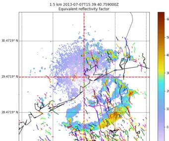
The final product can then be analyzed and plotted either spatially (as tracks, as in Fig. 3) or time series. For the work presented in this study the binary mask was constructed by thresholding each level of the grid at 35 dBZ. If any level for a given latitude–longitude is above that threshold, then the 2-D binary mask is marked as being part of a cell. Effectively this constitutes a 2-D projection of a 3-D binary field using a cascading AND operator.
A total of 3 years of KHGX data were processed (2015– 2017) using aforementioned techniques, mapped to a Carte-sian grid, and saved as CF-complaint NetCDF. Processing was parallelized by event, with events identified based on any radar grid exceeding a minimum reflectivity of 0 dBZ. Job scheduling and management was handled by the Dask li-brary (Dask, 2016). Over the 3 years, 7 TB of NEXRAD data
resulted in 20 MB of cell track data in a CSV file, yielding an efficient data reduction.
TINT tracks all convective cells. However, as we are in-terested in statistics of isolated cells, all TINT analyses pre-sented here include only isolated cells. A cell is considered isolated if it is not connected to any other cell by a contigu-ous path of grid cells exceeding a field threshold. Isolated cells therefore contain at most one peak field value.
3 Results
3.1 Observed case study cell evolution
Starting with the 8 June 2013 case study, Fig. 1 illustrates the routes of three observed features tracked using radarKDP
data, as well as the routes of three simulated features tracked using NU-WRFKDP. Most tracks are moving roughly
north-eastward, consistent with boundary layer onshore flow con-ditions. Both observed and simulated tracks are roughly 10– 20 km in distance. The only requirement for their selection was that they be isolated convective cells over land within 100 km of KHGX, such that cross sections exhibited no near neighbors on a subjective basis (as demonstrated below). Relatively few such cells were found in the observations or the simulation owing to lack of isolated cells developing or lack of developing cells remaining isolated, respectively. Al-though the somewhat disorganized convection observed ver-sus simulated differed, the tracking algorithm operating on KDPfields yielded satisfactory results for the purposes of this
pilot study.
Figure 3.An example of TINT-generated cell tracks from 7 July 2013 (randomly colored lines). A constant-altitude plot of reflectivity at 1.5 km is shown for reference. Each line showing the path of each cell is given a randomly generated cell identification number. The data are loaded into memory as a Pandas data frame and saved to a comma-separated variable file for later analysis.
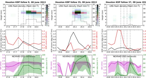
two dimensions of height and time. Here we see that cells 9 and 35 become electrically active roughly halfway through the track, and flashes are most concentrated between 8 and 10 km, just below the homogeneous freezing level (below the −40◦C level). Flash activity in cell 37 remains very weak
and is limited to elevations below 8 km. Cells 9 and 37 also show weak flash activity early in their tracks. We note that isolated flashes below the estimated melting level may be ar-tifacts of the processing algorithm used here, which could be refined in future work.
The second row of Fig. 4 shows two quantities calculated following Eq. (1), whereφ (z)is taken as the average value of KDPorZDRwithin 2.5 km of the track location. The
result-ingξ values, which we refer to as column strengths, allow a more robust measure of the featureKDPandZDRalong the
track than provided by the two-dimensional grids used by the tracking algorithm (in other words, a value applicable to the whole feature); we defer optimization of the averaging foot-print to future work beyond this pilot study. Since we found that the selected tracks follow relatively isolated and coherent reflectivity features in both the observations and the simula-tion (not shown), we also refer to the tracked features inter-changeably as cells and columns, with the understanding that the features tracked contain continuous peaks ofφ (z)at the resolution observed or simulated (otherwise they would not
have been tracked) but they do not necessarily correspond to individual isolated updrafts, however that may be defined. As shown in Fig. 4,KDPcolumn strength reaches sizable peaks
roughly halfway through the track in cells 9 and 35, but cell 37 shows no such peak. By contrast, all cells exhibit aZDR
column peak during the first half of their track, and that peak is greatest for cell 37. The robustness of theZDR column
strength appears indicative that all cells loft sufficiently large raindrops sufficiently far above the melting level to generate a strongZDRsignal (e.g., Kumjian et al., 2012; Snyder et al.,
2015).
The third row of Fig. 4 shows the median value and inner half of raindropDmvalues within 2.5 km of the track
loca-tion at all elevaloca-tions below the melting level, as well as rain rates retrieved at the lowest elevation angle (0.5◦). All cells show nearly continuous rain somewhere belowzmfrom track
start to end, as evidenced by the continuity ofDmretrievals,
but that rain does not reach the lowest scan elevation until at least 10 min after the start of each track. In cells 9 and 35, the near surface rain reaches peak rates during the second half of the track, beginning around the time that the KDP column
strength reaches its maximum. The considerable spread in surface rain rates indicates localized heavy rain that exceeds 100 mm h−1 in both cells. With the absence of aKDP
Figure 4.Time series from threeKDPcolumn objects tracked from observations show (top-to-bottom) lightning flashes per KHGX volume time (grey line) and occurrence density as a function of height (see color bar),KDPandZDRcolumn strength (calculated following Eq. 1), and retrieved rain rate and dropDm. Lightning and rain statistics collected within 2.5 km of the trackedKDPcolumn center. Vertical dashed lines indicate times of column 9 and 37 cross sections shown in Figs. 5 and 6.
rain rate maxima before and after itsZDRcolumn maximum.
The raindrop Dm is quite variable below all three tracked
columns, but the behavior seen in cell 9 appears for many tracked cells (not shown), namely,Dmincreasing withKDP
column strength and then plateauing at relatively high values along with decreased variance across the analyzed volume.
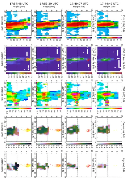
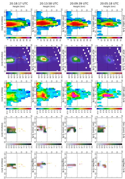
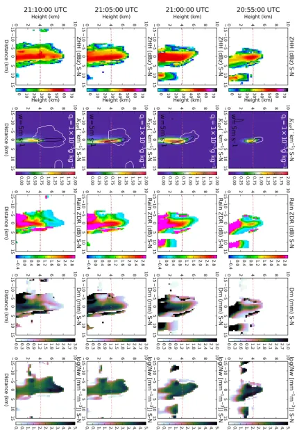
Figures 5 and 6 show four sequential north–south cross sections across the tracks of cells 9 and 37, which remain within similar distances from the radar (roughly 60 to 75 km; see Fig. 1), although cell 37 occurs roughly 2 h after cell 9. The cross-section times are indicated with vertical dotted lines in Fig. 4.
In cell 9 (Fig. 5), the first cross section corresponds to the time of peak ZDR and the last cross section corresponds to
the peak in electrical activity. The columns of Fig. 5 show ZHH,KDP,ZDR,Dm, and log(Nw), respectively, with
light-ning flashes overplotted in colors that indicate age from cur-rent to 10 min old. The first time shows the peak inZDR
col-umn strength, with elevated positive values (>1 dB) visible almost 3 km above the melting level. At this time the KDP
column is already visible, but lightning is absent. Within a rain shaft that is roughly 5–10 km in diameter,Dm is most
commonly greater than 1.8 mm andNw is most commonly
less than 300 mm−1m−3. The second time slices capture the peak of the KDP column strength, concurrent with the
be-ginning of electrical activity. Already at this point theZDR
column has decreased in height, with some evidence of neg-ativeZDRvalues associated with graupel or hail. By the third
time, scarcely anyZDRcolumn remains, but theKDPcolumn
remains visible and the lightning flash rate has intensified. By the fourth and last time, theKDPhas also largely
van-ished above the melting level. The lightning flash rate has not yet diminished in strength but flashes have lowered a bit in height (see also Fig. 4). The rain shaft has generally widened, with increasingly greater peak values of bothDm
and log(Nw) from track start to end.
In cell 37 (Fig 6), a vigorous ZDR column can be seen
initially. The diameters of the cell as measured by radar re-flectivity signal (roughly 10 km) and theZDRcolumn as
in-dicated by peak values (roughly 4 km) are similar to those of cell 9, but theZDR values are larger and the rain shaft
ap-pears weaker. However, in contrast to cell 9,KDP
enhance-ments are weak and almost isolated above the melting level at the first time. Retrieved rain parameters do not extend as high as seen in cell 9, consistent with a lower melting level that could be associated with its later time or more inshore location; owing to the absence of adequate meteorological observations, as discussed in Sect. 4, we assumed fixedzm
andzfvalues here. Within the rain shaft initially, occurrences
ofDmgreater than 2 mm are less common than in cell 9 and
Nwvalues are notably smaller. EnhancedKDPsubsequently
(roughly 15 min). At the third time, there is a sharp and local-ized peak of enhancedKDProughly 1 km below the melting
level, as in cell 9 at the third time shown, but the diameter of the region whereKDPexceeds 0.5◦km−1(often wider than
5 km) is roughly twice as great as that in cell 9 (roughly 3 km throughout). Perhaps related to the absence of a pronounced KDP column above the melting level, electrical activity
mains weak at all times in cell 37. The evolving rain shaft re-mains generally weaker than in cell 9, with generally smaller Dmand log(Nw).
A common pattern in observed tracked cells in this par-ticular case study is that first ZDR column strength peaks,
followed by KDP column strength, and then lightning
ac-tivity. However, cell 37 and other tracked cells that initiate northeast (downwind) of Houston exhibit the following devi-ations from that pattern: a greater leadingZDRpeak followed
by negligible KDPpeaks above the melting level and much
weaker lightning activity. According to satellite retrievals (see Fig. 1), the updraft cells in this latter class appear to exist within a region of generally more elevated aerosol concentra-tion than is found upwind or adjacent to the Houston plume flow. All else being equal, enhanced aerosol could at least initially lead to larger and fewer raindrops (e.g., Storer and van den Heever, 2013), potentially consistent with stronger ZDRand weakerKDPrain contributions in cell 37, whereas
cleaner conditions could at least initially lead to a more ac-tive warm rain process with more numerous and therefore smaller raindrops. Rain shaft retrievals do show generally smallerNwvalues below cell 37, consistent with fewer
rain-drops. There is some hint that Dmat the top of the cell 37
rain shaft at intermediate times shown may be larger than at the top of the cell 9 rain shaft, butDmvalues exceeding 2 mm
are clearly more common in cell 9, which produces consis-tently greater rain rates than cell 37 (see Fig. 4). We note that although electrification mechanisms and lightning pro-duction are not well understood, increased aerosol concen-trations have been more commonly associated with increased rather than decreased electrical activity (Murray, 2016, and references therein). Substantially more complex coupled mi-crophysical and dynamical pathways could also be primary contributors to both ZDR andKDP column evolution (e.g.,
Ryzhkov et al., 2011; Kumjian et al., 2014a; Snyder et al., 2015, and references therein). Owing to the short cell life cy-cles here, even basic and well observed factors such as height trends below the melting level (e.g., Kumjian and Prat, 2014) could be more indicative of time trends than quasi-steady properties. We defer robust analysis to future work, which would also need to address the role of meteorology, topog-raphy, observability (distance from radar), and other factors. Here we make the limited conclusion that such patterns in observed convective cells around Houston can be effectively identified and analyzed in an integrated fashion.
3.2 Simulated case study cell evolution
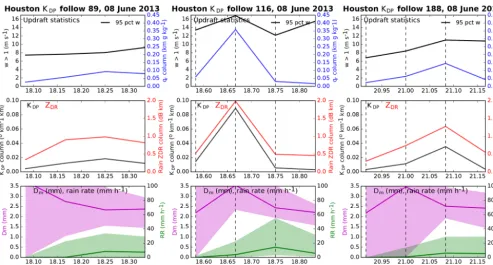
Figure 7 shows time series from three cells tracked from NU-WRF output in the same format as shown in Fig. 4 from observations. The times from track start to end for simu-lated cells 89, 116, and 188 are each roughly 25–30 min. The isolated cell tracks in the simulation are generally shorter than the isolated cell tracks in observations. Although many longer-lived cells were tracked in the simulation, they tended not to remain isolated. These general differences did not, however, hinder some basic comparisons of observed and simulated isolated cells as follows.
Since we did not attempt forward simulation of lightning flashes here, the first row of panels in Fig. 7 instead shows the 95th percentile of vertical wind speed (w) between the melting and freezing levels within 2.5 km of the track, which could potentially be retrieved from additional radar measure-ments in a future field campaign (e.g., Collis et al., 2013; North et al., 2017), and the column strength of supercooled qr. The second row of panels in Fig. 7 shows the time series
of column strengths ofKDPandZDRestimated from
simu-latedDm andNw (see Sect. 2). The third row of panels in
Fig. 7 shows the median value and inner half of raindropDm
values within 2.5 km of the track location at all elevations below the melting level, as well as rain rate at the surface.
All three simulated cells show surface rain beginning shortly after the track start and either declining or continu-ing after the track end time, as in observed cells, but the peak of median rain rates tends to be at least 5–10 times weaker than retrieved beneath observed cells. Despite weaker precip-itation, simulated raindropDmvalues are often near 2.5 mm,
greater than observed values often near 2 mm; we note that a fixed droplet number concentration of 100 cm−3was used in
the simulation (see Sect. 2) owing to the absence of aerosol size distribution measurements, which are discussed further in Sect. 4. Simulated cells show peaks ofqr,KDP, andZDR
column strength roughly collocated in time, consistent with the simplified use of supercooled rain properties to estimate the polarimetric quantities. SimulatedZDRcolumn strengths
are a bit greater than those observed, with variable peak val-ues of 1–2 dB km in each cell that are reached sometime during the inner half of the track duration. SimulatedKDP
column strengths are by contrast roughly an order of mag-nitude weaker than observed, consistent with the rain-based estimate ofKDP, resulting in underestimates aloft (Ryzhkov
et al., 2011) that are amplified by height weighting (Eq. 1). Whereas individual well-definedZDRpeaks tend to
consis-tently lead toKDP peaks in observations when the latter is
Figure 7.Time series from threeKDPcolumns tracked from NU-WRF simulation output show (top-to-bottom) updraft strength,qr,KDP, and ZDRcolumn strengths (calculated following Eq. 1), and rain rate and dropDmandNw. Updraft and rain statistics collected within 2.5 km of the trackedKDPcolumn center. Vertical dashed lines indicate times of columns 116 and 188 cross sections shown in Figs. 8 and 9.
whether a differingwstatistic than shown here is more cor-related. Simulated surface rain rate peaks with or shortly after theZDRcolumn strength, similar to observed cells.
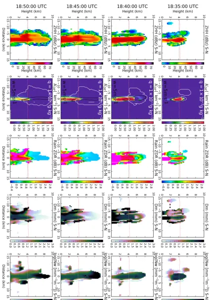
Figures 8 and 9 show north–south cross sections along the tracks of simulated cells 116 and 188 at the times in-dicated with vertical dotted lines in Fig. 7. In overall struc-ture, both simulated cells are 5–10 km in diameter and their 45 dBZ echoes reach at least 6–8 km, similar to the observed cells shown in Figs. 5 and 6. Simulated KDPstructures
ap-pear generally similar to those observed insofar as a single column is found at the center of each cell cross section, but the simulated columns exhibit substantially higher peak val-ues at column center (>1.75◦km−1) and do not decrease as rapidly with height. In the case of cell 116, higher peak val-ues abruptly decrease just below 6 km where rain appears to be rapidly frozen. The narrowness of simulatedqrcolumns
is more similar to observed cell 9 than 37.
In contrast to observations, there is a strong increase in simulated rainZDRandDmfrom the melting level to the
sur-face, an expected signature of raindrop size sorting that can be severely overestimated in two-moment bulk microphysics schemes such as that used here (Kumjian and Ryzhkov, 2010, 2012). The presence of mixed-phase particles complicates interpretation above the melting level. It can nonetheless be noted that simulated rainZDR greater than 2 dB reaches
5 km, as in both observed cells shown. Rain size distribution parameters shown from the mixed-phase region of the
sim-ulation, where they cannot be retrieved, indicate that weaker ZDRapproaching the homogeneous freezing level in cell 116
is associated with increasing rather than decreasingNw.
Sim-ulated cells commonly exhibit isolated and narrow regions of highZDRat supercooled temperatures on their north and
south flanks, similar to a less prominent feature on the north flank of observed cell 9.
3.3 Long-term statistics of cell occurrence
Using TINT as described in Sect. 2 enables a long-term sta-tistical analysis of isolated cell occurrence from KHGX ob-servations. From a 3-year climatology, Fig. 10 shows the total number of isolated cells that initiated as a function of month of the year. There is a pronounced period of enhanced oc-currence between June and September (approximately the summer months). This raises the question, is the increase in cells over the enhanced period due to an increased density of cells on a given day or more days with convective initiation events? Figure 11 shows the percentage of days in a given month with an initiation event within range of the KHGX radar. There is only a weak seasonal cycle, ranging from a 35 % chance of observing an isolated cell on a given day in December to just over 50 % on a given day in July, indicat-ing that the abrupt increase seen in June in Fig. 10 can be attributed to an increase in cell population density.
Figure 8.Sequential south–north cross sections from trackedKDPcolumn 116 show (left to right) calculatedZHH,KDPwith overplotted contours of updraft strength (w) greater than 5 m s−1and total ice mixing ratio (Qi) greater than 0.001 g kg−1,ZDR, and raindropDmand
Figure 10.Total number of isolated convective cells that initiated within a 200 km range of the KHGX radar during 2015–2017 by month.
Figure 11.Monthly percentage of days during 2015–2017 with at least one isolated cell initiation within a 200 km range of the KHGX radar.
function of time of day. The peak at a local time of 13:00 is consistent with a strong diurnal forcing. Furthermore, the lack of any apparent overnight maximum gives us confidence that we are effectively filtering out large-scale systems that have a nocturnal maximum (Nesbitt and Zipser, 2003).
The 2013 case study investigated above focused on ob-serving the microphysical and dynamical evolution of con-vective cells in a Lagrangian frame of reference. When in-vestigating the feasibility of deploying an agile radar sys-tem to Houston an important question arises: as a function of the radar’s unambiguous maximum range, how many cells will the radar see from initiation to dissipation? That is, how many full cell life cycles might the radar system collect? Fig-ure 13 shows the total number of cells as a function of the cell lifetime that would occur within 70, 150, and 200 km of a radar placed at the KHGX site during the enhanced oc-currence period. The totals are 441, 2442, and 4834 cells, respectively. If the assumption is made that the 3 years
stud-Figure 12. Total number of isolated cells that initiated within a 200 km range of the KHGX radar as a function of time of day dur-ing June through September of 2015–2017. The peak at 18:00 UTC corresponds to 13:00 local time.
Figure 13.Number of isolated cells that both initiated and dissi-pated with 70, 150, and 200 km of the KHGX radar as a function of cell lifetime during June through September of 2015–2017. Inte-grated totals are 441, 2442, and 4843, respectively.
ied are typical, we could therefore expect to see roughly 150, 800, and 1600 full life cycles in a single June through September deployment for a 70 km (e.g., X band), 150 km (C band), and 200 km (S band) radar range, scaling roughly with range area as would be expected if track density were geographically uniform.
Figure 14. Distribution of isolated cell initiation location during 2015–2017.
cells in the enhanced period might be expected to flow from a cleaner Gulf of Mexico air mass into a more polluted Hous-ton air mass. This quirk of climatology suggests that the en-hanced period convection lends itself well to studying the impact of aerosols on isolated, precipitating convective cells.
4 Conclusions and discussion
The comparison of tracked cells from Houston NEXRAD ob-servations and a NU-WRF simulation demonstrates the po-tential value of polarimetric weather radar observations for systematically observing and improving the understanding and simulation of convective cell physics. Factors related to the meteorological and aerosol environment, such as the structure of rain size distribution parameters below the melt-ing level, are particularly well suited to analysis usmelt-ing such data. Above the melting level, further investigation of the microphysical properties controlling KDP and ZDR
signa-tures is likely to yield additional quantitative constraints on simulation physics; comparing observations with forward-simulated values from well-observed case studies is likely to yield substantial progress, especially using an integrative approach that also considers rain properties below the melt-ing level and overall cell structural evolution. Future simu-lations could employ bin microphysics or other approaches to avoid errors associated with sedimentation or hydrome-teor size distribution shape, as well as mixed-phase particle representation to improve forward simulation of polarimet-ric signatures (e.g., Ryzhkov et al., 2011; Kumjian et al., 2014a; Snyder et al., 2017a; Matsui et al., 2018b). Forward simulation of lightning flash rates (e.g., Barthe et al., 2010; Basarab et al., 2015) may be simultaneously compared with collocated LMA observations to study the correlations of up-draft physics and flash rate signatures such as those shown in Fig. 4.
However, cell tracking in both KHGX observations and a simulation also demonstrates the potential value of improved
Figure 15.Directional cumulative distribution of propagation direc-tion during June through October versus November through May.
spatiotemporal resolution that could be achieved using mo-bile research radars. Isolated cell cores are relatively poorly resolved and their evolution is rapid compared with the KHGX operational volume scan rate.KDPandZDRcolumns
associated with updraft cores rise and fall within 10–15 min time spans, as shown in Figs. 4 and 7. Similar conclusions have been reached in past studies (e.g., Loney et al., 2002). Future simulations can obtain arbitrarily higher spatial res-olution and output timing, whereas radar measurements are subject to cell distance from the radar and, in this study, the fixed scanning strategies of the operational weather radar. For the purposes of studying isolated convection around Hous-ton, we conclude that substantial value could be added by mobile research radars that could achieve higher resolution and faster scan rates (e.g., Isom et al., 2013; Pazmany et al., 2013; Snyder et al., 2013; Kumjian et al., 2014b). Stein et al. (2015) demonstrate the value of applying a statistical ap-proach to convective cells that are tracked in simulations and in radar observations using an adaptive rapid scan strategy. Sufficient radar resources to perform wind vector retrievals (e.g., Collis et al., 2013; North et al., 2017) could supply ob-servations adequate to statistically study the relationship of cell microphysics and updraft strength.
of the radar according to the statistics collected in our 3-year sample. Finally, cells observed would have a dominant propagation vector just west of southerly, indicating that cells forming along the shoreline would likely experience aerosol perturbations corresponding to their proximity to emission sources.
The demanding objectives of a box flux closure experi-ment (Rosenfeld et al., 2014) would require meteorological measurements at high spatiotemporal resolution at all do-main boundaries, but even for the more limited study of up-draft physics investigated here as an amendment to such a campaign, we note that routine meteorological data are lack-ing in the Houston region. The nearest operational sound-ings are at Lake Charles and Corpus Christi, roughly 200 km to the northeast and 300 km to the southwest, respectively. Obtaining soundings during convective activity, ideally at more than one site within the KHGX domain, would pro-vide a foundation required to establish atmospheric structure, which is of first-order importance to convective cell devel-opment. To the extent that improving model physics is an objective, it would be imperative to collect observations that are adequate to demonstrate that simulations reproduce basic properties of atmospheric structure. The capability of state-of-the-art regional models to reproduce basic atmospheric structure should not be assumed a given even when using an assimilation-informed data set for inputs at domain bound-aries. Owing to the relatively rapid evolution of the diurnal boundary layer properties with time and distance from the coastline under the target conditions of onshore flow, ground-based in situ and remote-sensing measurements capable of establishing boundary layer height and water vapor mixing ratio would also add great value.
Finally, in situ measurements remain the most robust means of observing cloud-active aerosol properties from the surface to the middle free troposphere. At a minimum, sur-face measurements of boundary layer CCN spectra and to-tal aerosol number concentration measurements from ideally more than one location in the KHGX domain would allow a means of constraining at least boundary layer fields. To avoid the challenge and expense of a long aircraft campaign, past aircraft measurements from recent field campaigns in the Houston region could provide statistical guidance on ex-pected discontinuities at the boundary layer top (e.g., Lance et al., 2009). Measurement of INPs from at least one surface site would add substantial value; we are aware of no past INP measurements in the Houston region.
Code availability. Py-ART is available from http://arm-doe.github. io/pyart/ (last access: 28 May 2019). Trackpy is available from http: //soft-matter.github.io/trackpy/v0.3.2/ (last access: 28 May 2019). TINT is available from https://github.com/openradar/TINT (last ac-cess: 28 May 2019). NU-WRF is available from http://nuwrf.gsfc. nasa.gov/ (last access: 28 May 2019).
log10f (Dm)= −5.98+6.64log10Dm−1.28(log10Dm)2,
(A3) with Dm in millimeters, Nw in reciprocal cubic meters
per millimeter, and KDP in degrees per kilometer.
Author contributions. DR provided CCN retrievals and selected suitable case study dates. MvLW prepared KHGX data with assis-tance from SG and SC. MP is the lead software engineer for TINT and was assisted by RJ. TM and AF prepared the NU-WRF simula-tion and outputs. AR and PZ provided rain retrievals. DM and RW provided lightning mapping array data. MvLW, AF, SC, MP, and RJ prepared analyses and figures. AF, SC, MvLW, and XL prepared the paper.
Competing interests. The authors declare that they have no conflict of interest.
Acknowledgements. This work was partially supported by the Of-fice of Science (BER), U.S. Department of Energy, under agree-ment DE-SC0006988, and by the NASA Radiation Sciences Pro-gram. NU-WRF is supported by the NASA Modeling, Analysis and Prediction (MAP) program. Resources supporting this work were provided by the NASA High-End Computing (HEC) Pro-gram through the NASA Advanced Supercomputing (NAS) Di-vision at Ames Research Center and NASA’s Center for Climate Simulation (NCCS) at Goddard Space Flight Center. The contri-bution of Scott Collis through Argonne National Laboratory was supported by the U.S. Department of Energy, Office of Science, Of-fice of Biological and Environmental Research, under contract DE-AC02-06CH11357. We gratefully acknowledge the computing re-sources provided on Blues and Bebop, a high-performance comput-ing cluster operated by the Laboratory Computcomput-ing Resource Cen-ter at Argonne National Laboratory. Johannes Quaas co-organized the Aerosol, Cloud, Precipitation and Climate initiative workshop at the NASA Goddard Institute for Space Studies in April 2015, where this work was conceived with the additional participation of Jiwen Fan, Corinna Hoose, Philip Stier, Bastiaan van Diedenhoven, and Shuguang Wang. A companion regional model intercomparison study of another case study date is being led by Sue van den Heever (http://acpcinitiative.org, last access: 28 May 2019). Results of this pilot study were used to inform design of the Tracking Aerosol Convection Interactions Experiment (TRACER) field campaign (https://www.arm.gov/research/campaigns/amf2021tracer, last ac-cess: 28 May 2019).
Review statement. This paper was edited by Gianfranco Vulpiani and reviewed by two anonymous referees.
References
Ackerman, A. S., Fridlind, A. M., Grandin, A., Dezitter, F., Weber, M., Strapp, J. W., and Korolev, A. V.: High ice water content at low radar reflectivity near deep convection – Part 2: Evaluation of microphysical pathways in updraft parcel simulations, Atmos. Chem. Phys., 15, 11729–11751, https://doi.org/10.5194/acp-15-11729-2015, 2015.
Barthe, C., Deierling, W., and Barth, M. C.: Estimation of total lightning from various storm parameters: A cloud-resolving model study, J. Geophys. Res., 115, D24202, https://doi.org/10.1029/2010JD014405, 2010.
Basarab, B. M., Rutledge, S. A., and Fuchs, B. R.: An im-proved lightning flash rate parameterization developed from Colorado DC3 thunderstorm data for use in cloud-resolving chemical transport models, J. Geophys. Res., 120, 9481–9499, https://doi.org/10.1002/2015JD023470, 2015.
Blahak, U., Zeng, Y., and Epperlein, D.: Radar forward operator for data assimilation and model verification for the COSMO-model: Preprint of 35th Conf. on Radar Meteorology, Amer. Meteor. Soc., Pittsburgh, PA, P10.119, 2011.
Bosilovich, M. G., Akella, S., Coy, L., Cullather, R., Draper, C., Gelaro, R., Kovach, R., Liu, Q., Molod, A., Norris, P., Wargan, K., Chao, W., Reichle, R., Takacs, L., Vikhliaev, Y., Bloom, S., Collow, A., Firth, S., Labow, G., Partyka, G., Pawson, S., Reale, O., Schubert, S., and Suarez, M.: MERRA-2: Initial Evaluation of the Climate, NASA/TM-2015-104606, in series: Technical Report Series on Global Modeling and Data Assimilation, vol. 43, 145 pp., 2015.
Bringi, V. N., Liu, L., Kennedy, P. C., Chandrasekar, V., and Rut-ledge, S. A.: Dual multiparameter radar observations of intense convective storms: The 24 June 1992 case study, Meteorol. At-mos. Phys., 59, 3–31, 1996.
Bringi, V. N. and Chandrasekar, V.: Polarimetric Doppler Weather Radar: Principles and Applications, Cambridge University Press, Cambridge, UK, 636 pp., 2001.
Chou, M.-D. and Suarez, M. J.: A solar radiation parameteriza-tion for atmospheric studies, NASA//TM-1999-10460, vol. 15, 38 pp., 1999.
Chou, M.-D. and Suarez, M. J.: A thermal infrared radiation param-eterization for atmospheric studies, NASA/TM-2001-104606, in series: Technical Report Series on Global Modeling and Data As-similation, vol. 19, 55 pp., 2001.
Collis, S., Protat, A., May, P. T., and Williams, C.: Statistics of storm updraft velocities from TWP-ICE including verification with profiling measurements, J. Appl. Meteorol. Climatol., 52, 1909–1922, https://doi.org/10.1175/JAMC-D-12-0230.1, 2013. Dask Development Team: Dask: Library for dynamic task
schedul-ing, available at: https://dask.org/ (last access: 28 May 2019), 2016.
DeMott, P. J., Prenni, A. J., Liu, X., Kreidenweis, S. M., Petters, M. D., Twohy, C. H., Richardson, M. S., Eidhammer, T., and Rogers, D. C.: Predicting global atmospheric ice nuclei distributions and their impacts on climate, P. Natl. Acad. Sci. USA, 107, 11217– 11222, https://doi.org/10.1073/pnas.0910818107, 2010. Dixon, M. and Wiener, G: TITAN: Thunderstorm identification,
tracking, analysis and nowcasting – A radar-based methodology, J. Atmos. Ocean. Tech., 10, 785–797, 1993.
Du, R., Du, P., Lu, Z., Ren, W., Liang, Z., Qin, S., Li, Z., Wang, Y., and Fu, P.: Evidence for a missing source of efficient ice nuclei, Sci. Rep., 7, 39673, https://doi.org/10.1038/srep39673, 2017. Fan, J., Leung, L. R., Rosenfeld, D., Chen, Q., Li, Z.,
Zhang, J., and Yan, H.: Microphysical effects determine macrophysical response for aerosol impacts on deep convec-tive clouds, P. Natl. Acad. Sci. USA, 110, E4581–E4590, https://doi.org/10.1073/pnas.1316830110, 2013.
observa-mos. Chem. Phys., 17, 5947–5972, https://doi.org/10.5194/acp-17-5947-2017, 2017.
Giangrande, S. E., McGraw, R., and Lei, L.: An application of linear programming to polarimetric radar differential phase processing, J. Atmos. Ocean. Tech., 30, 1716–1729, 2013.
Hallett, J. and Mossop, S. C.: Production of secondary ice particles during the riming process, Nature, 249, 26–28, 1974.
Helmus, J. J. and Collis, S. M.: The Python ARM Radar Toolkit (Py-ART), a library for working with weather radar data in the Python programming language, J. Open Res. Software, 4, e25, https://doi.org/10.5334/jors.119, 2016.
Herbert, R. J., Murray, B. J., Dobbie, S. J., and Koop, T.: Sensitivity of liquid clouds to homogenous freezing pa-rameterizations, Geophys. Res. Lett., 42, 1599–1605, https://doi.org/10.1002/(ISSN)1944-8007, 2015.
Homeyer, C. R. and Kumjian, M. R.: Microphysical characteristics of overshooting convection from polarimetric radar observations, J. Atmos. Sci., 72, 870–891, 2015.
Hubbert, J., Bringi, V. N., Carey, L. D., and Bolan, S.: CSU-CHILL polarimetric radar measurements from a severe hail storm in east-ern Colorado, J. Appl. Meteorol., 37, 749–775, 1998.
IPCC: The IPCC Scientific Assessment, in: Report Prepared for In-tergovernmental Panel on Climate Change by Working Group I, edited by: Houghton, J. T., Jenkins, G. J., and Ephraums, J. J., Cambridge University Press, Cambridge, UK, 410 pp., 1990. IPCC: Climate Change 2013: The Physical Science Basis, in:
Con-tribution of Working Group I to the Fifth Assessment Report of the Intergovernmental Panel on Climate Change, edited by: Stocker, T. F., Qin, D., Plattner, G.-K., Tignor, M., Allen, S. K., Boschung, J., Nauels, A., Xia, Y., Bex, V., and Midgley, P. M., Cambridge University Press, Cambridge, UK and New York, NY, USA, 1535 pp., 2013.
Isom, B., Palmer, R., Kelley, R., Meier, J., Bodine, D., Yeary, M., Cheong, B.-L., Zhang, Y., Yu, T.-Y., and Biggerstaff, M. I.: The atmospheric imaging radar: Simultaneous volumet-ric observations Using a phased array weather radar, J. Atmos. Ocean. Technol., 30, 655–675, https://doi.org/10.1175/JTECH-D-12-00063.1, 2013.
Jakob, C. and Tselioudis, G.: Objective identification of cloud regimes in the tropical western Pacific, Geophys. Res. Lett., 30, 2082, https://doi.org/10.1029/2003GL018367, 2003.
Johnson, J. T., Mackeen, P. L., Witt, A., Mitchell, D. W., Stmpf, G. J., Eilts, M. D., and Thomas, K. W.: The storm cell identifica-tion and tracking algorithm: An enhanced WSR-88D algorithm, Weather Forecast., 13, 263–276, 1998.
the polarimetric radar variables, J. Atmos. Sci., 69, 2042–2060, https://doi.org/10.1175/JAS-D-11-0125.1, 2012.
Kumjian, M. R., Ganson, S. M., and Ryzhkov, A. V.: Freez-ing of raindrops in deep convective updrafts: A microphys-ical and polarimetric model, J. Atmos. Sci., 69, 3471–3490, https://doi.org/10.1175/JAS-D-12-067.1, 2012.
Kumjian, M. R. and Prat, O. P.: The impact of raindrop collisional processes on the polarimetric radar variables, J. Atmos. Sci., 71, 3052–3067, https://doi.org/10.1175/JAS-D-13-0357.1, 2014. Kumjian, M. R., Khain, A. P., Benmoshe, N., Ilotoviz, E., Ryzhkov,
A. V., and Phillips, V. T. J.: The anatomy and physics ofzDR columns: Investigating a polarimetric radar signature with a spec-tral bin microphysics model, J. Appl. Meteorol. Climatol., 53, 1820–1843, 2014.
Kumjian, M. R., Rutledge, S. A., Rasmussen, R. M., Kennedy, P. C., and Dixon, M.: High-resolution polarimetric radar observations of snow-generating cells, J. Appl. Meteorol. Climatol., 53, 1636– 1658, https://doi.org/10.1175/JAMC-D-13-0312.1, 2014. Ladino, L. A., Korolev, A., Heckman, I., Wolde, M., Fridlind,
A. M., and Ackerman, A. S.: On the role of ice-nucleating aerosol in the formation of ice particles in tropical mesoscale convective systems, Geophys. Res. Lett., 44, 1574–1582, https://doi.org/10.1002/2016GL072455,2017.
Lakshmanan, V. and Smith, T.: An objective method of evaluating and devising storm-tracking algorithm, Weather Forecast., 25, 701–709, 2010.
Lance, S., Nenes, A., Mazzoleni, C., Dubey, M. K., Gates, H., Varutbangkul, V., Rissman, T. A., Murphy, S. M., Sorooshian, A., Flagan, R. C., Seinfeld, J. H., Feingold, G., and Jonsson, H. H.: Cloud condensation nuclei activity, clo-sure, and droplet growth kinetics of Houston aerosol dur-ing the Gulf of Mexico Atmospheric Composition and Cli-mate Study (GoMACCS), J. Geophys. Res., 114, D00F15, https://doi.org/10.1029/2008JD011699, 2009.
Lawson, R. P., Woods, S., and Morrison, H.: The microphysics of ice and precipitation development in tropical cumulus clouds, J. Atmos. Sci., 72, 2429–2445, https://doi.org/10.1175/JAS-D-14-0274.1, 2015.
Limpert, G., Houston, A., and Lock, N.: The advanced algorithm for tracking objects (AALTO), Meteor. Apps., 22, 694–704, https://doi.org/10.1002/met.1501, 2015.
MacGorman, D. R., Rust, W. D., Schuur, T. J., Biggerstaff, M. I., Straka, J. M., Ziegler, C. L., Mansell, E. R., Bruning, E. C., Kuhlman, K. M., Lund, N. R., Biermann, N. S., Payne, C., Carey, L. D., Krehbiel, P. R., Rison, W., Eack, K. B., and Beasley, W. H.: TELEX: The Thunderstorm Electrification and Lightning Exper-iment, B. Am. Meteorol. Soc., 89, 997–1013, 2008.
Matsui, T., Zhang, S. Q., Tao, W.-K., Lang, S., Ichoku, C., and Peters-Lidard, C.: Impact of radiation frequency, precipitation ra-diative forcing, and radiation column aggregation on convection-permitting west African monsoon simulations, Clim. Dynam., https://doi.org/10.1007/s00382-018-4187-2, online first, 2018a. Matsui, T., Dolan, B., Rutledge, S., Tao, W.-K., Iguchi, T.,
Barnum, J., and Lang, S.: POLARRIS: Polarimetric Radar Retrievals and Instrumental Simulator, J. Geophys. Res., https://doi.org/10.1029/2018JD028317, online first, 2018b. Mauritsen, T. and Stevens, B.: Missing iris effect as a
pos-sible cause of muted hydrological change and high cli-mate sensitivity in models, Nature Geosci., 8, 346–351, https://doi.org/10.1038/ngeo2414, 2015.
McKinney, W.: Data Structures for Statistical Computing in Python, in: Proceedings of the 9th Python in Science Conference, edited by: van der Walt, S. and Millman, J., 51–56, 2010.
Morrison, H., Thompson, G., and Tatarskii, V.: Impact of cloud mi-crophysics on the development of trailing stratiform precipitation in a simulated squall line: Comparison of one- and two-moment schemes, Mon. Weather Rev., 137, 991–1007, 2009.
Murray, L. T.: Lightning NOxand impacts on air quality: Curr. Poll. Rep., 2, 115–133, https://doi.org/10.1007/s40726-016-0031-7, 2016.
Nakanishi, M. and Niino, H.: Development of an improved turbu-lence closure model for the atmospheric boundary layer, J. Me-teor. Soc. Jpn., 87, 895–912, 2009.
Nesbitt, S. W. and Zipser, E. J.: The Diurnal Cycle of Rain-fall and Convective Intensity according to Three Years of TRMM Measurements, J. Climate, 16, 1456–1475, https://doi.org/10.1175/1520-0442-16.10.1456, 2003.
NOAA: National Weather Service (NWS) Radar Operations Cen-ter: NOAA Next Generation Radar (NEXRAD) Level 2 Base Data, NOAA National Centers for Environmental Information, https://doi.org/10.7289/V5W9574V, 1991.
NOAA: 88D meteorological observations, Part C, WSR-88D products and algorithms, Federal Meteorological Handbook 11, Report FCM-H11C-2017, Office of the Federal Coordinator for Meteorological Services and Supporting Research, 394 pp., 2017.
North, K. W., Oue, M., Kollias, P., Giangrande, S. E., Collis, S. M., and Potvin, C. K.: Vertical air motion retrievals in deep convective clouds using the ARM scanning radar network in Oklahoma during MC3E, Atmos. Meas. Tech., 10, 2785–2806, https://doi.org/10.5194/amt-10-2785-2017, 2017.
Orville, R. E., Cullen, M. R., Rodeheffer, D., Krehbiel, P. R., and Rison, W.: The Houston Lightning Mapping Array: Installation, operation, and preliminary results, AGU Fall Meeting Abstracts, 2012.
Pazmany, A. L., Mead, J. B., Bluestein, H. B., Snyder, J. C., and Houser, J. B.: A mobile rapid-scanning X-band polarimet-ric (RaXPol) Doppler radar system, J. Atmos. Ocean. Tech., 30, 1398–1413, https://doi.org/10.1175/JTECH-D-12-00166.1, 2013.
Peters-Lidard, C. D., Kemp, E. M., Matsui, T., Santanello, Jr., J. A., Kumar, S. V., Jacob, J. P., Clune, T., Tao, W.-K., Chin, M., Hou, A., Case, J. L., Kim, D., Kim, K.-M., Lau, W., Liu, Y., Shi, J., Starr, D., Tan, Q., Tao, Z., Zaitchik, B. F., Za- vodsky, B., Zhang, S. Q., and Zupanski, M.: Integrated modeling of aerosol, cloud, precipitation and land processes at satellite-resolved scales, Environ. Model. Softw., 67, 149–159, https://doi.org/10.1016/j.envsoft.2015.01.007, 2015.
Pope, M., Jakob, C., and Reeder, M. J.: Objective classification of tropical mesoscale convective systems, J. Climate, 22, 578–5808, 2009.
Pruppacher, H. R. and Klett, J. D.: Microphysics of Clouds and Pre-cipitation, 2nd edn., Kluwer Academic Publishers, 954 pp., 1997. Reichle, R. H., Koster, R. D., De Lannoy, G. J. M., Forman, B. A., Liu, Q., Mahanama, S. P. P., and Toure, A.: Assessment and enhancement of MERRA land surface hydrology estimates, J. Climate, 24, 6322–6338, https://doi.org/10.1175/JCLI-D-10-05033.1, 2011.
Rosenfeld, D., Andreae, M. O., Asmi, A., Chin, M., de Leeuw, G., Donovan, D. P., Kahn, R., Kinne, S., Kivekäs, N., Kul-mala, M., Lau, W., Schmidt, K. S., Suni, T., Wagner, T., Wild, M., and Quaas, J.: Global observations of aerosol-cloud-precipitation-climate interactions, Rev. Geophys., 52, 750–808, https://doi.org/10.1002/2013RG000441, 2014.
Rosenfeld, D., Zheng, Y., Hashimshoni, E., Pöhlker, M. L., Jefferson, A., Pöhlker, C., Yu, X., Zhu, Y., Liu, G., Yue, Z., and Fischman, B.: Satellite retrieval of cloud con-densation nuclei concentrations by using clouds as CCN chambers, P. Natl. Acad. Sci. USA, 113, 5828–5834, https://doi.org/10.1073/pnas.1514044113, 2016.
Rossow, W. B., Tselioudis, G., Polak, A., and Jakob, C.: Tropical climate described as a distribution of weather states indicated by distinct mesoscale clour property mixtures, Geophys. Res. Lett., 32, L21812, https://doi.org/10.1029/2005GL024584, 2005. Ryzhkov, A., Pinsky, M., Pokrovsky, A., and Khain, A.:
Po-larimetric radar observation operator for a cloud model with spectral microphysics, J. Appl. Meteorol. Climatol., 873–894, https://doi.org/10.1175/2010JAMC2363.1, 2011.
Ryzhkov, A., Diederich, M., Zhang, P., and Simmer, C.: Potential utilization of specific attenuation for rainfall estimation, mitiga-tion of partial beam blockage, and radar networking, J. Atmos. Ocean. Tech., 31, 599–619, https://doi.org/10.1175/JTECH-D-13-00038.1, 2014.
Scharenbroich, L., Nagnusdottir, G., Smyth, P., Stern, H., and Wang, C.-C.: A Bayesian framework for storm tracking using a hidden-state representation, Mon. Weather Rev., 138, 2132– 2148, 2010.
Sherwood, S. C., Bony, S., and Dufresne, J.-L.: Spread in model climate sensitivity traced to atmospheric convective mixing, Na-ture, 505, 37–42, https://doi.org/10.1038/nature12829, 2014. Snyder, J. C., Bluestein, H. B., Venkatesh, V., and Frasier, S. J.:
Observations of polarimetric signatures in supercells by an X-band mobile Doppler radar, Mon. Weather Rev., 141, 3–29, https://doi.org/10.1175/MWR-D-12-00068.1, 2013.
17-9599-2017, 2017.
Stein, T. H. M., Hogan, R. J., Clark, P. A., Halliwell, C. E., Han-ley, K. E., Lean, H. W., Nicol, J. C., and Plant, R. S.: The DYMECS project: A statistical approach for the evaluation of convective storms in high-resolution NWP models, B. Amer. Me-teorol. Soc., 96, 939–951, https://doi.org/10.1175/BAMS-D-13-00279.1, 2015.
Storer, R. L. and van den Heever, S. C.: Microphysical processes ev-ident in aerosol forcing of tropical deep convective clouds, J. At-mos. Sci., 70, 430–446, https://doi.org/10.1175/JAS-D-12-076.1, 2013.
Tan, I., Storelvmo, T., and Zelinka, M. D.: Observational constraints on mixed-phase clouds imply higher climate sensitivity, Science, 352, 224–227, https://doi.org/10.1126/science.aad5300, 2016. Testud, J., Oury, S., Black, R., Amayenc, P., and Dou, X.: The
con-cept of “normalized” distribution to describe raindrop spectra: A tool for cloud physics and cloud remote sensing, J. Appl. Meteo-rol., 40, 1118–1140, 2001.
Thurai, M., Bringi, V. N., Carey, L. D., Gatlin, P., Schultz, E., and Petersen, W. A.: Estimating the accuracy of polarimetric radar-based retrievals of drop-size distribution parameters and rain rate: An application of error variance separation using radar-derived spatial correlations, J. Hydrometeorol., 13, 1066–1079, https://doi.org/10.1175/JHM-D-11-070.1, 2012.
Vali, G., DeMott, P. J., Möhler, O., and Whale, T. F.: Technical Note: A proposal for ice nucleation terminology, Atmos. Chem. Phys., 15, 10263–10270, https://doi.org/10.5194/acp-15-10263-2015, 2015.
van Lier-Walqui, M., Fridlind, A. M., Ackerman, A. S., Collis, S., Helmus, J. J., North, K., Kollias, P., MacGorman, D. R., and Pos-selt, D. J.: On polarimetric radar signatures of deep convection for model evaluation: columns of specific differential phase ob-served during MC3E, Mon. Weather Rev., 144, 737–758, 2016.
Wang, S., Sobel, A. H., Fridlind, A., Feng, Z., Comstock, J. M., Minnis, P., and Nordeen, M. L.: Simulations of cloud-radiation interaction using large-scale forcing derived from the CINDY/DYNAMO northern sound-ing array, J. Adv. Model. Earth Syst., 7, 1472–1498, https://doi.org/10.1002/2015MS000461, 2015.
Yano, J.-I. and Phillips, V. T. J.: Ice-ice collisions: An ice multiplica-tion process in atmospheric clouds, J. Atmos. Sci., 68, 322–333, https://doi.org/10.1175/2010JAS3607.1, 2011.
Zhang, J., Qi, Y., Tang, L., Cocks, S., Wang, Y., Zhang, P., Ryzhkov, A., Langston, C., and Kaney, B.: MRMS dual-polarization radar synthetic QPE, 38th Conference on Radar Meteorology, Chicago, IL, Amer. Meteor. Soc., 22B.3, 2017.
Zipser, E. J.: Some views on “hot towers” after 50 years of tropi-cal field programs and two years of TRMM data, in: Cloud Sys-tems, Hurricanes, and the Tropical Rainfall Measuring Mission (TRMM), edited by: Tao, W.-K. and Adler, R., American Mete-orological Society, 49–58, 2003.
Zrni´c, D. S. and Ryzhkov, A. V.: Polarimetry for weather surveillance radars, B. Am. Meteorol. Soc., 80, 389–406, https://doi.org/10.1175/1520-0477(1999)080<0389:PFWSR>2.0.CO;2, 1999.