https://doi.org/10.5194/amt-12-3151-2019 © Author(s) 2019. This work is distributed under the Creative Commons Attribution 4.0 License.
Can liquid cloud microphysical processes be used for vertically
pointing cloud radar calibration?
Maximilian Maahn1,2, Fabian Hoffmann1,3, Matthew D. Shupe1,2, Gijs de Boer1,2, Sergey Y. Matrosov1,2, and Edward P. Luke4
1Cooperative Institute for Research in Environmental Sciences (CIRES), University of Colorado Boulder,
Boulder, Colorado, USA
2NOAA Earth System Research Laboratory (ESRL), Physical Sciences Division, Boulder, Colorado, USA 3NOAA Earth System Research Laboratory (ESRL), Chemical Sciences Division, Boulder, Colorado, USA 4Brookhaven National Laboratory, Upton, New York, USA
Correspondence:Maximilian Maahn ([email protected]) Received: 16 January 2019 – Discussion started: 30 January 2019
Revised: 10 May 2019 – Accepted: 13 May 2019 – Published: 13 June 2019
Abstract. Cloud radars are unique instruments for observ-ing cloud processes, but uncertainties in radar calibration have frequently limited data quality. Thus far, no single ro-bust method exists for assessing the calibration of past cloud radar data sets. Here, we investigate whether observations of microphysical processes in liquid clouds such as the transi-tion of cloud droplets to drizzle drops can be used to cal-ibrate cloud radars. Specifically, we study the relationships between the radar reflectivity factor and three variables not affected by absolute radar calibration: the skewness of the radar Doppler spectrum (γ), the radar mean Doppler veloc-ity (W), and the liquid water path (LWP). For each relation, we evaluate the potential for radar calibration. Forγ andW, we use box model simulations to determine typical radar re-flectivity values for reference points. We apply the new meth-ods to observations at the Atmospheric Radiation Measure-ment (ARM) sites North Slope of Alaska (NSA) and Oliktok Point (OLI) in 2016 using two 35 GHzKa-band ARM Zenith
Radars (KAZR). For periods with a sufficient number of liq-uid cloud observations, we find that liqliq-uid cloud processes are robust enough for cloud radar calibration, with the LWP-based method performing best. We estimate that, in 2016, the radar reflectivity at NSA was about 1±1 dB too low but sta-ble. For OLI, we identify serious problems with maintaining an accurate calibration including a sudden decrease of 5 to 7 dB in June 2016.
1 Introduction
Due to their profiling capabilities, millimeter wavelength cloud radars are one of the most important tools for cloud re-mote sensing. Their measurements are used for process stud-ies as well as for long-term monitoring of hydrometeor prop-erties. Although maintaining an accurate radar calibration is absolutely crucial to avoid biases and false trends in observa-tional data sets, calibrating cloud radars accurately is a chal-lenging and long-standing problem. In this study, we investi-gate the potential for using observations of liquid cloud mi-crophysical processes for radar calibration.
magni-tude in power and – particularly for pulsed radars – the span between the transmitted and received power is even larger.
The community has multiple approaches for calibrating cloud radars but none are applicable to all situations. Most commonly, a budget calibration is done wherein all compo-nents are calibrated separately and the individual calibration constants are summed (Chandrasekar et al., 2015). A budget calibration can also be combined with a receiver calibration by observing a reference target emitting microwave radia-tion. For example, Whiton et al. (1977) proposed pointing a scanning radar into the sun and Küchler et al. (2017) used liquid nitrogen – similar to the standard calibration method of microwave radiometers. Yet, the errors of the individual budget calibrations sum up, and there is a risk of overlook-ing error sources, e.g., due to an interaction between radar components. Therefore, it is advantageous to calibrate the full radar system end-to-end. Atlas (2002) provided an ex-tensive overview of different end-to-end radar calibration techniques, most of them relying on observing objects with known radar cross sections. These reference targets included corner reflectors and various metallic or metallized spherical objects such as ping pong balls, ball projectiles from air guns, and Christmas ornaments. However, observations of refer-ence targets require dedicated field operations and cannot be used to calibrate past data sets. Also, the observation of a reference target with radar can be challenging for a number of reasons. First, most reference targets do not move, and hence do not cause a Doppler shift; thus, the target’s return cannot be distinguished from ground clutter unless the target is positioned far away from the surface. For lifting the target from the surface, past studies proposed using fiberglass poles (Kollias et al., 2016), tethered balloons (Atlas and Mossop, 1960), or unmanned aerial vehicles (Küchler et al., 2017). Second, the exact location of the target with respect to the radar needs to be known for calibration because reference targets are point targets. Instead, atmospheric hydrometeors are volume distributed targets. Third, the antenna properties are not well defined unless the target is in the antenna’s far-field, i.e., at least a couple of hundred meters away from the radar. Lastly, receiver saturation must be avoided, which re-quires the use of an attenuator or a sufficient distance be-tween the calibration target and the radar. Because of these reasons, calibration by reference targets is only feasible for scanning cloud radars but not for vertically pointing cloud radars, which are most commonly used.
Several studies have suggested calibrating radars by com-paring their measurements of rainfall with integrated drop size distributions from ground-based disdrometers (Joss et al., 1968; Ulbrich and Lee, 1999; Frech et al., 2017). Tri-don et al. (2017) proposed using self-consistency checks of retrievals from simultaneous radar observations at multiple frequencies to identify calibration problems. However, dis-drometers and regular liquid precipitation are required for monitoring calibration continuously and the challenge of radome or antenna attenuation during precipitation events
needs to be considered, particularly for vertically pointing systems.
If multiple radars are available, it is easier to achieve a rel-ative calibration by cross-calibration. Cross-calibration also works when the radars have different frequencies, as long as the hydrometeors are small enough to assume Rayleigh scat-tering and differential attenuation is accounted for (Hogan et al., 2000; Kneifel et al., 2015; Ewald et al., 2019). If the radars are not collocated, the cross-calibration can also be done statistically by comparing long-term data sets. But such comparisons can be biased by different radar sensitivities and it is important to degrade both radars to the same sen-sitivity. Protat et al. (2011) compared observations statisti-cally from the CloudSat satellite W-band radar with ground-based observations for relative calibration. Because Cloud-Sat’s calibration is well established (Tanelli et al., 2008), Pro-tat et al. (2011) and Louf et al. (2019) proposed using Cloud-Sat as a reference for absolute calibration of ground-based radars. However, long time series of at least several months are required (Kollias et al., 2019) and the method cannot be used to monitor radar calibration at higher temporal resolu-tions. Merker et al. (2015) proposed another method for ab-solute radar calibration of radars by intercomparisons, but their method requires a very specific setup with three small radars.
We can also avoid the problem of absolute radar calibra-tion by using variables not affected by absolute calibracalibra-tion, such as the higher moments of the radar Doppler spectrum (Maahn et al., 2015), attenuation (Matrosov, 2005) and some polarimetric variables such as depolarization ratio (Matrosov et al., 2017), differential reflectivity, and differential phase shift (Oue et al., 2018). Yet, excluding variables reduces the information content of the observations significantly (Maahn and Löhnert, 2017) depending on the application.
In summary, no method for obtaining an absolute calibra-tion is available that works in all situacalibra-tions. Either dedicated field campaigns or in situ observations of drop size distri-butions are required. Budget calibrations are not end-to-end, and relative calibrations require trusting the calibration of a reference radar. To close this gap, we investigate whether liq-uid cloud microphysical processes can be used for radar cal-ibration. Luke and Kollias (2016) proposed using the unique relationship between the equivalent radar reflectivity factor (here referred to as reflectivity orZe, in dBz, Smith, 2010)
and the skewness of the radar Doppler spectrum (γ, unit-less) during drizzle onset – commonly defined as drops ex-ceeding the critical diameter for starting autoconversion (20 to 40 µm) – for calibration. Several studies have suggested thatγis helpful for studying drizzle formation (Kollias et al., 2011a, b; Luke and Kollias, 2013; Acquistapace et al., 2019). Further, Luke and Kollias (2016) suggested that the relation-ship between the liquid water path (LWP, in kg m−2) and the maximum reflectivity in the column max(Ze) contains
drops to grow larger by condensation and enhance the prob-ability of drizzle formation leading to higherZevalues (see
Fig. 1 of Acquistapace et al., 2019). In this study, we evaluate whether the Ze–γ and LWP–max(Ze) relationships can be
used for calibrating vertically pointing cloud radars. In addi-tion to these two relaaddi-tionships proposed by Luke and Kollias (2016), we also investigate the relationship betweenZeand
the mean vertical Doppler velocity (W, in m s−1) becauseW has been successfully used for drizzle detection (e.g., Shupe, 2007) due to the larger fall velocity of drizzle drops.
We run box model simulations of drizzle onset to develop the details of the method, characterize its uncertainties, and apply it to radar observations of the North Slope of Alaska (NSA) and Oliktok Point (OLI) ARM sites from 2016. The instruments, data sets, box model, and radar simulator used in this study are detailed in Sect. 2. The calibration meth-ods used in this study are presented in Sect. 3. Besides the three new methods based on liquid cloud microphysical pro-cesses, we use a reference method to calibrate the two cloud radars relative to one another. For this, we modify the relative calibration method that Protat et al. (2011) proposed for cali-brating ground-based cloud radars with CloudSat. In Sect. 4, we apply the various calibration methods to data from NSA and OLI and assess the temporal evolution of the calibration quality at both sites. Finally, concluding remarks are given in Sect. 5.
2 Data sets and models 2.1 Sites
In this study, we use ground-based remote sensing observa-tions from two observatories operated by the DOE ARM pro-gram located in northern Alaska: Utqia˙gvik (ARM’s North Slope of Alaska, NSA site, formerly known as Barrow, 71.323◦N, 156.616◦W) and Oliktok Point (OLI, 70.495◦N, 149.886◦W). While the former was established in 1996, the latter did not become fully operational until late 2015. Both sites are located on the coast of the Beaufort Sea and lie only 250 km apart. The synoptic-scale forcing is very sim-ilar, resulting in high correlations between both sites for sea level pressure and near-surface air temperature, humidity, and wind (Maahn et al., 2017).
2.2 Instruments and observations
Both sites are equipped with a 35 GHzKa-band ARM Zenith
Radar (KAZR). While the radar at NSA is a first-generation KAZR, the one at OLI is a second-generation KAZR2 with improved sensitivity (Table 1). The spectral resolution of the OLI KAZR2 was increased from 256 to 512 Doppler spec-tral bins on 16 June 2016. For the radar moments Ze, γ,
andW, we use the radar product presented in Williams et al. (2018), which, unlike the standard ARM general mode (GE) moment products, includes advanced clutter removal and
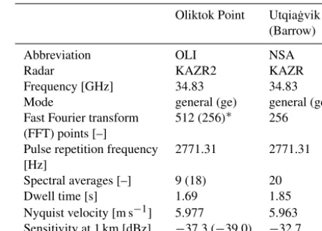
Table 1.Technical specifications of the radars at Oliktok Point and Utqia˙gvik (Barrow).
Oliktok Point Utqia˙gvik (Barrow)
Abbreviation OLI NSA
Radar KAZR2 KAZR
Frequency [GHz] 34.83 34.83 Mode general (ge) general (ge) Fast Fourier transform 512 (256)∗ 256 (FFT) points [–]
Pulse repetition frequency 2771.31 2771.31 [Hz]
Spectral averages [–] 9 (18) 20 Dwell time [s] 1.69 1.85 Nyquist velocity [m s−1] 5.977 5.963 Sensitivity at 1 km [dBz] −37.3 (−39.0) −32.7
∗Specifications in parentheses correspond to the configuration before
16 June 2016.
higher moments such asγ (Williams, 2018). Because turbu-lence can mask microphysical signals inγ, observations with high temporal resolution are usually required for minimizing broadening effects of the Doppler spectrum (Acquistapace et al., 2017). Instead, Williams et al. (2018) use a shift-then-average method to reduce the impact of turbulence on the radar moments, allowing the use of coarser temporal resolu-tion (15 s). For temperature and humidity profiles, we use the standard ARM interpolated radiosonde product (ARM user facility, 1999) based on three (two) daily launches at NSA (OLI). Further, both sites are equipped with ceilome-ters for cloud base estimation (Vaisala CL31, ARM user fa-cility, 1996) and microwave radiometers (MWRs) to retrieve LWP and integrated water vapor (IWV) using the MicroWave Radiometer RETrieval (MWRRET, Turner et al., 2007) and the Monochromatic Radiative Transfer Model (MonoRTM; Clough et al., 2005). To minimize MWR retrieval biases, we applied monthly offset corrections to the observed brightness temperatures using MonoRTM to forward model clear-sky radiosonde observations. At NSA, we estimate LWP from a combination of the 90 GHz channel of an RPG-150-90 ra-diometer (ARM user facility, 2006, the 150 GHZ channel was not operational in 2016) and the 23.8 and 31.4 GHz channels of a Radiometrics WVR-1100 radiometer (ARM user facility, 1993). At OLI we retrieve LWP from a three-channel (23.834, 30, and 89 GHz) Radiometrics PR2289 ra-diometer (ARM user facility, 2011). For identifying cloud phase, we use the phase classification by Shupe (2007), which depends on a combination of KAZR, MWR, radioson-des, and micropulse lidar (MPL, ARM user facility, 1990) measurements.
The site at OLI was also equipped with aKa-band
ver-tically for only 10 min h−1. Combined with its reduced sen-sitivity, this leads to too few observations of liquid clouds, and thus we decided not to include KaSACR observations in this study.
Unless stated otherwise, Ze is corrected for gaseous
at-tenuation (Rosenkranz, 1998) using the radiosonde profiles scaled by the MWR’s IWV. Two-way integrated gaseous at-tenuation is typically less than 0.4 dB for the whole vertical column at the Ka-band. Attenuation by liquid water is
ne-glected.W is adjusted to sea level air density following Za-wadzki et al. (2005).
We analyze observations of the full year 2016 obtained at both sites. The time period was selected because the KAZR at OLI became fully operational only in fall 2015 and suf-fered from a malfunction of a phase-lock oscillator resulting in resonance peaks in the Doppler spectrum for most of 2017. 2.3 Box model
To simulate the transition from cloud droplets to drizzle drops in an idealized way, we use a zero-dimensional box model of the droplet collection process (Hoffmann et al., 2017). The box model results will allow us to determine the potential of using drizzle onset for radar calibration. The box model is based on the “superdroplet” approach, in which several hundred computational particles are simulated, each superdroplet representing an ensemble of real, identical droplets. We apply the so-called “all-or-nothing” approach to calculate collections among the superdroplets, which has been shown to accurately represent collision–coalescence in the superdroplet framework (Unterstrasser et al., 2017). The model is initialized using the so-called “singleSIP” method (Unterstrasser et al., 2017). In this method, the underly-ing droplet size distribution is divided into logarithmically spaced bins. Each bin is represented by one superdroplet, of which the diameter and weighting factor (the number of real droplets represented by that superdroplet) are determined by integrating the droplet size distribution across the bin. Here, we use 500 bins, i.e., 500 superdroplets, to represent the droplet size distribution.
While we also use measured droplet size distributions, we primarily use an idealized lognormal drop size distribution (Feingold and Levin, 1986) to evaluate the sensitivity of our calibration methods by varying the distribution’s parameters systematically:
N (D)=√ Ntot 2πln(σg)D
exp
−ln2(D/d
g)
2ln2(σg)
, (1)
with D the droplet diameter, Ntot the total number of
droplets, dg the geometric mean diameter, and σg the
geo-metric standard deviation.
Collision–coalescence is steered by the collection kernel, in which the droplet velocity difference is calculated using terminal velocities by Beard (1976), the collision
efficien-cies are taken from Hall (1980), coalescence efficiency is assumed as unity, and turbulent enhancement is described as in Ayala et al. (2008) and Wang and Grabowski (2009). Turbulence enhancement of the collision process is con-trolled by a prescribed energy dissipation rate (see Riechel-mann et al., 2012). The simulation time has been restricted to 3 h. Note that no other microphysical processes besides collision–coalescence are considered, and droplets are not al-lowed to sediment from the box; i.e., the liquid water content (LWC) remains constant (Hoffmann et al., 2017).
2.4 Radar simulator
To convert the drop size distributions (DSDs) of the box model into radar observables, we use the spectral radar simu-lator of the second-generation Passive and Active Microwave radiative TRAnsfer model (PAMTRA2; as in Maahn and Ori, 2019). Its physical basics are the same as for the first-generation PAMTRA (Maahn et al., 2015; Maahn and Löhn-ert, 2017), but it is designed in a more modular way. Because the drop size in the box model does not exceed 1/10th of the radar wavelength (8.6 mm) forZe<10 dBz, we can use
the Rayleigh scattering assumption for estimating the radar backscattering cross section of the drops. From the backscat-tering cross section, the radar Doppler spectrum is estimated using the same fall-velocity–size relationship as in the box model (Beard, 1976). Unlike forZe andW, broadening by
the Doppler spectrum due to turbulence imposing random motion on the droplets needs to be accounted for when es-timatingγ. For this, we convolve a Gaussian velocity distri-bution with the idealized radar spectrum. The standard de-viation of the Gaussian distribution depends mostly on the degree of turbulence and the contribution of the horizon-tal wind field to the radial velocity due to the finite radar beamwidth following Shupe et al. (2008). The former is esti-mated from the energy dissipation rate, which is varied as discussed below, and a constant horizontal wind of 10 m s−1 is assumed for the latter. Noise is added to the spectrum in correspondence with KAZR2 specifications after June 2016 (Table 1). From the simulated radar Doppler spectrum, we estimate its moments including radar reflectivityZe, mean
Doppler velocityW, and skewnessγ following Maahn and Löhnert (2017).
3 Calibration methods
3.1 Skewness and mean Doppler-velocity-based methods
We hypothesize that there are reference points during drizzle onset that have a typicalZevalue, which can be constrained
– referred to as autoconversion – we assume that collision– coalescence is the dominating cloud process during drizzle onset and that other cloud processes can be neglected for this purpose. To assess the model’s sensitivity to the micro-physical properties of a given cloud, we first vary the initial DSDs (Sect. 3.1.1). Based on these results, we determine the best reference points for radar calibration (Sect. 3.1.2) and discuss how to apply these reference points to observations (Sect. 3.1.3).
3.1.1 Sensitivity study
Here, we show how Ze,γ, andW change with time during
drizzle onset and how this is affected by the DSD and turbu-lence. For a reference run, we chose a set of parameters fea-turing a slow cloud-to-drizzle transition in agreement with observations of DSDs (Geoffroy et al., 2010) and turbulence (Shupe et al., 2012; Maahn et al., 2015):Ntot=108m−3as
the initial drop number, σg=1.34 as the standard
geomet-ric deviation,dg=1.6×10⁻⁵m as the geometric mean
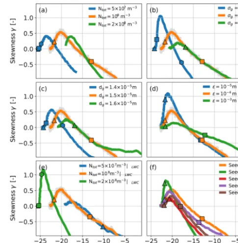
di-ameter to describe the initial lognormal distribution (Eq. 1), and=10−4m2s−3as the turbulent energy dissipation rate. This DSD corresponds to 0.26 g m−3 LWC. The results of the reference run show (orange lines Fig. 1) that Ze
in-creases monotonically with time and thatγ reflects the typ-ical competition of cloud droplets and drizzle drops in the radar Doppler spectrum (Kollias et al., 2011b). In the absence of drizzle, only backscattering by cloud droplets contributes to the radar Doppler spectrum. For this stage, the Doppler spectrum has a Gaussian shape (i.e., γ≈0), the variability of droplet fall velocities is small, and turbulence regulates the width of the Doppler spectrum. The critical droplet diameter required to start autoconversion varies between 14 and 80 ×10−6m depending on the DSD (Liu et al., 2004). As soon as the first drizzle drops are created by autoconversion after 45 min, the γ values become positive (motion towards the radar is defined as positive in this study) because the drizzle drops extend the tail of the Doppler spectrum towards faster, more positive velocities. The maximumγ value of approxi-mately 0.7 is reached at−20.2 dBz (referred to asZmax(γ )e in
the following). When drizzle and cloud droplets contribute approximately equally to Ze, the shape of the spectrum is
again more symmetric resulting in γ≈0. This stage is re-ferred to as the cloud drizzle balance point in the follow-ing and is reached after another 45 min at −16.5 dBz (re-ferred to as Zγe=0). Finally,γ becomes negative when the
spectrum is dominated by drizzle drops and the remaining cloud droplets extend the tail of the spectrum to the opposite, smaller-droplet side. However, simulated values significantly larger thanZeγ=0have to be treated with care because drizzle
removal from the cloud by sedimentation is not accounted for by the box model.
To assess the sensitivity of theZe–γ relationship to
mi-crophysics, the initial parameters of the box model were per-turbed. We chose the perturbations such that a realistic range
is covered but made sure that drizzle is created neither in-stantly nor too slowly (i.e., no drizzle after 3 h runtime). To evaluate the sensitivity with respect toNtot, we divided and
multipliedNtotby a factor of 2 (Fig. 1a). When cloud droplets
dominate the radar signal,Ntotscales linearly withZein
lin-ear units and the offset between the model runs is close to 3 dB (corresponding to a factor of 2 as expected from the modification ofNtot). Consequently, theZemax(γ )values are
approximately 3 dB apart (−23.5, −20.2, and −17.6 dBz). However, autoconversion is more efficient for greater num-ber concentrations (with constant droplet size), thusγ de-creases faster as a function of bothZeand time than for the
other runs. Due to these compensating effects,Zeγ=0values
are closer together (−16.5 and−15.4 dBz) than for the max-imum ofγ. Interestingly, this is not the case if we reduce Ntotby 50 %. Then, theZe–γline is shifted to the lower left
andZeγ=0is−21.1 dBz and 4.7 dB smaller than for the
ref-erence run. For this run, autoconversion is so slow that after 2 h cloud droplets still dominate the spectrum and a reflec-tivity value of only−15 dBz is reached at the end of the 3 h simulation. For the run with doubledNtot, the time required
until the drizzle dominates the radar Doppler spectrum (i.e., γ <0) is less than 1 h.
For estimating the sensitivity to the width of the size dis-tribution, we perturbσgby±0.05 (Fig. 1b). If we perturbed
the initial DSD width by larger values, the box model would create drizzle too slowly or too quickly for our purposes. While theZmax(γ )e values for both perturbations are about
2 dB apart, the difference between the Zeγ=0 values is 2.9
and 0.2 dB for the reduction and increase inσg, respectively.
Similar to the doubledNtot run, autoconversion is more
ef-ficient and faster when we increaseσg. At the same time, a
narrower distribution leads to a larger absoluteγ value due to the reduced Doppler spectrum width of the cloud peak. Note that the reference run and the run with increased σg
are almost identical forZe>−18 dBz, but the run with
re-ducedσgremains different. This highlights that the presence
of larger droplets in the initial spectrum (due to a larger stan-dard deviation) is important for drizzle onset, but the effect saturates when drizzle drops become more numerous. This is similar for the runs wheredghas been increased and reduced
by±1 µm (Fig. 1c).Zγe=0changes little when increasingdg
(−16.3 dBz) but is reduced for a smallerdg(−19.4 dBz).
To assess the impact of turbulence on drizzle onset,is perturbed by an order of magnitude (Fig. 1d), in agreement with observations of Arctic clouds (Shupe et al., 2012). En-hanced turbulence leads to turbulent broadening, which re-duces theγ magnitude by making the spectrum more sym-metrical (Acquistapace et al., 2017). This is particularly vis-ible for low reflectivities, which are dominated by cloud droplets. Turbulence only has a small impact on autocon-version, which can be seen by the slightly faster drizzle for-mation and the small change inZeγ=0of 0.2 dB. Similar
(2017), in which turbulence did not significantly change the timing of drizzle but rather the amount of cloud water trans-formed to drizzle.
In reality, a change inNtot alone is not very realistic
be-cause whenNtotis increased, the available liquid is typically
distributed on a larger number of smaller sized droplets. In other words, an increase inNtotfor fixed LWC, which would
shift theZe–γ relationship towards largerZevalues, is
com-pensated for by a reduction ofdg, which would shift the
re-lationship to the opposite direction. To investigate this, we repeated the Ntot variation for fixed LWC by changing dg
accordingly (Fig. 1e). Note that the required change in dg
is larger (18.9 and 11.9 µm) than investigated above. As ex-pected, autoconversion is more efficient in the lowNtot|LWC
case, but there is apparently an upper threshold for Zγe=0,
which increases only by 1 dB. For the high Ntot|LWC case,
Zγe=0is reduced strongly from−16.5 to−22.9 dBz. Unlike
for the other runs, drizzle formation is very slow and droplets still dominate after 2 h of model run time. Interestingly, the steeper slope of theZe–γ relationship for the highNtot|LWC
case agrees with the results of Kollias et al. (2011a), who compared maritime and continental (implying higher Ntot
values) data sets.
Collision–coalescence, including autoconversion, is a stochastic process so a random number generator is used in the box model for emulation. To make sure the runs are com-parable, we previously seeded the random number genera-tor with the same number for the sensitivity study. Here, we use five different seeds for the reference initial DSD to quan-tify the role of chance. Figure 1f shows thatZeγ=0(Z
max(γ )
e )
varies significantly between −16.5 and−18.9 dBz (−20.0 and−21.6 dBz). We conclude from this that the stochastic nature of collision–coalescence reduces the impact of the clouds’ initial DSD on theZe–γ relationship. However, the
impact of stochasticity is likely overestimated in the box model because of the limited number of simulated super-droplets (Dziekan and Pawlowska, 2017).
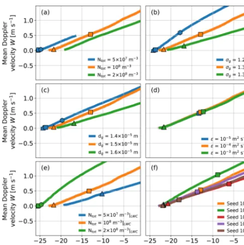
For comparison, we also evaluate the results of the sensi-tivity study with respect to theZe–W relationship (Fig. 2).
Generally,Wincreases with increasing drizzle concentration because the drop fall velocity depends strongly on size. On the one hand,W is more prone to biases thanγ, e.g., due to inaccurate radar pointing or vertical air motion. While we as-sume that the latter cancels for longer time series, consistent lifting related to orography could biasW even for long-term data sets. On the other hand,W can be found in radar data sets more frequently than γ and observingW does not re-quire a high temporal resolution (Acquistapace et al., 2017). The dependence on the initial DSD is similar to the Ze–γ
relationship. The fact that drizzle develops more efficiently for DSDs with larger Ntot,σg, or dg can be seen from the
slowerW for the sameZe. This is becauseW (proportional
to the first DSD moment for drizzle) increases more slowly with size thanZe(proportional to the sixth DSD moment).W
Figure 1.Sensitivity of the reflectivityZeto skewnessγtransition
for drizzle onset to(a)total number concentrationNtot,(b)the
unit-less standard deviation of the lognormal distributionσg,(c)the
ge-ometric mean diameterdg, and(d)the turbulent energy dissipation
rate. We also(e)modifiedNtotwhile keeping liquid water content
(LWC) constant (i.e., increasingdg) and(f)used different seeds for
the box model. All lines are smoothed. The light gray points show all data points of the reference run; the lines denote smoothed model results. The triangles, squares, and hexagonal shapes indicate model simulation times of 1, 1.5, and 2 h, respectively. Note that the orange lines are identical for all panels.
does not depend on; therefore, the runs with differentare practically identical. Unlike forZeγ=0, there are apparently
no saturation effects limiting the variability of theZe–W
re-lationship.
3.1.2 Determining reference values
The sensitivity study evaluated only a single microphysical condition, which is not realistic for observations. Therefore, we investigate how stable the relations are for longer data sets with varying microphysical conditions and assess whether theZe–γ andZe–W relations have the potential to be used
for radar calibration. For this, we used the box model and combined all perturbations ofNtot,σg,dg, andwith each
Figure 2.As in Fig. 1 but for mean Doppler velocityW.
The results show considerable spread forσandW(Fig. 3) thus we were able to obtained a median relationship. For this, we bin the data byZe(bin width 1 dB) and estimate the
me-dian values of γ andW for every bin. We smooth the re-sulting curve using the Savitzky–Golay filter (window length 7, polynomial order 2, Savitzky and Golay, 1964). That is particularly important when applying the method to obser-vations (see below) because it makes the method more ro-bust by increasing the number of observations contributing to a particular point on the curve. Typically, the smoothing changes Zeγ=0 by less than 1 dB. The resulting median
re-lationships show the typical partly sinusoidally shapedZe–
γ relationship and an increase inW forZe>−20 dBz. We
maintain that this median curve is much better suited for cali-bration because the mean reflectivity would be more sensitive to outliers. It is important to consider the wholeZe–γ
rela-tionship instead of determining a mean value for allZewith
γ =0. This is because a certainσ value is not unambigu-ous and, e.g., a value of γ=0 can also refer to a spectrum consisting only of cloud droplets.
To determine which point of theZe–γandZe–Wrelations
is most stable and best suited for calibration, we estimate the uncertainties of severalZereference values forγ(maximum,
0,−0.1) andW (0.25,0.5,0.75 m s−1) for comparison. The choice of the reference values is somewhat arbitrary, but the variability increases strongly outside the investigated range of reference values, which enclose the onset of drizzle. While the determination of max(γ) is straightforward, we estimate the other values by linear interpolation from the neighboring Zebins. In case a reference point is crossed more than once
by the median relationship (e.g.,γ of cloud droplets is also
close to zero), we choose the crossing associated with a larger Ze value. The use of the Savitzky–Golay filter ensures that
adjacentZe bins impact the reference values, which makes
the method more stable. Unlike otherZecalibration studies
(e.g., Protat et al., 2011), we do not need to account for radar sensitivity differences because the range of relevantZe
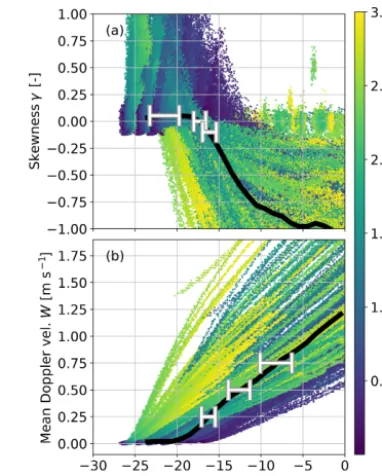
val-ues is strictly limited and well above the sensitivity limit. To assess the stability of the reference values, we use a boot-strapping approach: we select 5 % of the 340 runs randomly 100 times and determine the resulting reference values for each subset. We estimate the final reference values and their uncertainties from the means and standard deviations, re-spectively (see uncertainty bars in Fig. 3). Forγ, the com-parison reveals that the variability ofZeis less for reference
γvalues 0 and−0.1 (±0.7 and 0.8 dB, Table 2) than for the maximum ofγ (±1.6). ForW, the variability is generally larger (±0.8 to 1.9 dB).
Even though we chose the initial conditions to be represen-tative of liquid stratiform clouds at high latitudes, it is possi-ble that our choice of initial conditions is biased. Therefore, we repeated the box model experiment with initial conditions based on aircraft in situ observations from the same region as the cloud radars expecting that measured DSDs include all microphysical processes including advection and sedimen-tation (Fig. 4). For this, we use data of the 5th ARM Air-borne Carbon Measurements (ACME-V) aircraft campaign. This campaign took place from June to September 2015 and included cloud probe observations near the North Slope of Alaska (ARM user facility, 2016). Here, we use liquid-only cloud observations in the vicinity of OLI and NSA. We use every 10th profile of the data shown in the Fig. 4a and b of Maahn et al. (2017). Except for the initial DSDs, the setup is identical to the idealized runs introduced above. was not measured during ACME-V and we apply the same values as for the sensitivity study to each measured profile (=10−3, 10−4, and 10−5m2s−3). Every run was repeated five times with different seeds; runs that did not produce drizzle or that included drizzle in the initial DSD were not considered. By doing so, we avoid the impact of potential sampling problems of large, rare drizzle drops by the in situ probes. This leaves 237 runs and the bootstrapping method is used to determine the uncertainties of the reference points. Even though the estimatedZe–γandZe–Wrelationships are
more uneven, the general shape between−20 and−10 dBz is very similar to the runs using lognormal DSDs (Table 2).
Figures 3 and 4 contain only box model runs where drizzle eventually formed, but the minimum requiredZefor drizzle
formation is different for ACME-V data than for the ideal-ized DSDs. While for the idealideal-ized DSDs drizzle is formed only whenZeof the initial DSD is at least−27 dBz, drizzle
enhancedγ values below−20 dBz. This is most likely only a spin-up effect of the box model, which can be seen from the excellent agreement of the median curves for largerZe.
Note also that at−21 dBzγ is around zero due to competi-tion between runs with higher and lowerγ values. But this does not bias our calibration method because we only use the crossing with the largestZevalue.
For both initial DSDs, the variability determined from bootstrapping is minimal forγ =0.0 and W=0.25 m s−1, and we conclude that Zγe=0 andZW=0.25e are the best
ref-erence values for assessing radar calibration. Initializing the simulations with the lognormal and ACME-V DSDs,Zγe=0is −17.3±0.7 and−17.8±1.2, respectively (Table 2).ZeW=0.25 is estimated as −16.3±0.8 and −16.9±1.5 dBz, respec-tively. Combining both setups, we obtainZeγ=0= −17.6 and
ZWe =0.25= −16.6 dBz. These values are very close to the value of−17 dBz proposed by Frisch et al. (1995) for distin-guishing between drizzle-free and drizzle-containing clouds. Given the idealized setup, we likely underestimated the un-certainties ofZγe=0andZWe =0.25and estimate the uncertainty
to be at least 3 dB.
While it is true that we found a much larger variability ofZγe=0andZWe =0.25 for the sensitivity study (Sect. 3.1.1),
we are confident that the reference values can still be deter-mined with sufficient accuracy. We base this claim on the as-sumption that observations with reflectivities corresponding to drizzle onset (Ze−20 to−15 dBz) are likely dominated by
clouds that produce drizzle slowly. Clouds with faster driz-zle production reach larger reflectivities quickly, likely have a shorter lifetime, and do not contribute to the data set quan-titatively. Clouds without or with extremely slow autoconver-sion rates will likely not reachZevalues larger than−20 dBz
before the end of their lifetime. Together with the signifi-cant role of random effects, this indicates that the variability of the Ze–γ andZe–W relationships for larger data sets is
lower than estimated in the sensitivity study. By binning the box model results byZeand determining the medianγ and
W values, we ensure that slow drizzle generating clouds also dominate our box model estimates because, similar to obser-vations, clouds forming drizzle quickly in the box model also have quickly increasingZe values. Therefore, these clouds
contribute little to observations of reflectivities between−20 and−15 dBz.
This does not mean that Zeγ=0 andZeW=0.25 can be used
to identify individual profiles with or without drizzle. As shown in the sensitivity study above and in Acquistapace et al. (2019), the variability from profile to profile can be substantial andZe,γ, and W are not suited to identify the
presence of drizzle for individual profiles. 3.1.3 Application to observations
In the following, we determine Zeγ=0 and ZeW=0.25 from
observations at NSA and OLI. Comparison with the
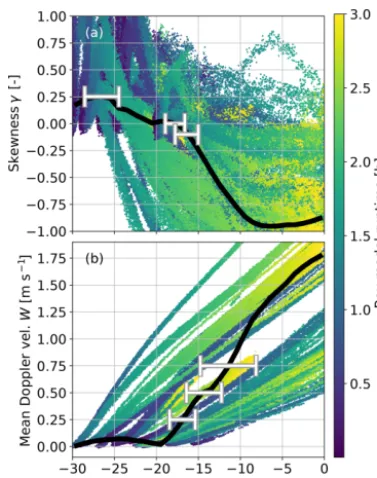
theo-Figure 3. (a)Reflectivity Ze skewnessγ and(b) reflectivityZe
mean Doppler velocityW relationships for the individual model runs using synthetic initial model conditions. The black lines denote the medians as a function ofZe; the error bars are estimated using
bootstrapping for selectedγ andWvalues (see Table 2). Color is for model run time.
Table 2.MeanZevalues at various reference points forγ andW.
Reference value idealizedZe[dBz] ACME-VZe[dBz]
max(γ) −21.3±1.6 −26.6±2.0 γ=0.0 −17.3±0.7 −17.8±1.2 γ= −0.1 −16.1±0.8 −16.4±1.4 W=0.25 m s−1 −16.3±0.8 −16.9±1.5 W=0.50 m s−1 −12.6±1.3 −14.3±2.1 W=0.75 m s−1 −8.2±1.9 −11.4±3.3
retical values derived above will allow for evaluating the radars’ calibration. We only use clouds identified by the Shupe (2007) method as purely liquid throughout the col-umn. We expect that drizzle onset can be observed best in stratiform clouds due to their lower turbulence, and we limit our analysis to observations with a cloud base lower than 1000 m and cloud thickness less than 1000 m. Even though the Doppler spectrum peak identification algorithm provided by Williams et al. (2018) can identify atmospheric signals with a signal-to-noise ratio (SNR) as small as−15 dB, we only use data with SNR>−5 dB becauseγ is a particularly noisy variable. We use the same method to estimateZγe=0
Figure 4.As in Fig. 3 but using ACME-V observations as the initial conditions.
medianγ andW values are estimated for each bin, and the resulting curve is smoothed using the Savitzky–Golay filter. Bins with fewer than 100 observations are omitted from the analysis. To obtainZγe=0andZeW=0.25, the median
relation-ships are interpolated linearly.
3.2 Liquid-water-path-based method
Here, we investigate the potential of the relation between LWP andZefor calibration. While the relationships between
γ orW andZeare shaped by the drizzle onset process, the
correlation between LWP and Ze is based on the fact that
the likelihood of drizzle formation (i.e., increasedZevalues)
increases with increasing LWP. But there is also a correla-tion between LWP and Ze for non-drizzling clouds: cloud
droplets can grow larger in deeper clouds with greater LWP values. Frisch et al. (1998) showed that for non-drizzling adiabatic clouds with constantNtot, LWP is proportional to
P
iz 1/2
i withzi=10
Ze,i/10for range gatei. While this rela-tionship could be exploited for radar calibration assuming a fixedNtotvalue, we were not able to apply the method to our
data set successfully. This is likely due to challenges identify-ing a sufficient number of clouds fulfillidentify-ing the conditions of the method (i.e., non-drizzling adiabatic clouds with constant Ntot). Instead, we decided to use the maximum Ze value in
the column (max(Ze)) to combine the one-dimensional LWP
with the two-dimensional, range-resolvedZemeasurements.
Not relying on the relationship found by Frisch et al. (1998) allows us to not distinguish between non-drizzling and driz-zling clouds and use the very same data set as for theγ and Wmethods. Even though max(Ze) is likely noisier than, e.g.,
the mean ofZein the column, max(Ze) has the major
advan-tage that the maximum is less likely impacted by radar sen-sitivity than the mean because a truncation of a distribution’s lower end does not impact its maximum.
3.2.1 Determining a reference relation
Similar to theZe–γ andZe–W relationships, and as shown
for cloud-integrated reflectivity by Frisch et al. (1998), the LWP–max(Ze) relationship likely also depends on
micro-physical (e.g., initialNtot) and dynamical (e.g., turbulence,
entrainment and mixing) conditions. With respect to the LWP–max(Ze) relationship, we expect that higherNtot
val-ues lead to reducedZevalues for the same LWP due to
sup-pression of drizzle formation. But unlike theγ- andW-based methods, which focus on a very specific moment during driz-zle onset, the LWP method is impacted by the full set of pro-cesses of droplet growth and drizzle formation, and is po-tentially impacted by multiple feedback processes between clouds and their environment. For example, the impact of Ntoton the LWP–max(Ze) relationship would be even larger
assuming drizzle suppression due to enhancedNtotleads to
larger LWP values (Albrecht, 1989). However, the question of whether and how feedback processes compensate for a LWP increase is still debated (Stevens and Feingold, 2009). Focusing only on drizzle onset has allowed us to use a simple box model to determine the reference points for theZe–γand
Wrelationships but addressing the question of howNtot(and
the related cloud condensation nuclei concentration) changes LWP cannot be answered with a box model and is beyond the scope of this study. Therefore, we decided not to use a model for determining a reference LWP–max(Ze) relationship.
In-stead, we will use the LWP–max(Ze) relationship of one site
as a reference and determine the calibration offset of a second site from this. In other words, the LWP–max(Ze) relationship
is used in a relative way unless we can trust the calibration of one of the radars, which would make it an absolute cali-bration similar to Protat et al. (2011). Similar to theγ- and W-based methods, this assumes that the LWP–max(Ze)
rela-tionship is sufficiently stable with respect to changes in mi-crophysical and dynamical conditions. Because we have no box model to identify the LWP value with the lowest vari-ability of max(Ze), we do not use a reference point but a
reference relationship and minimize the mean weighted dif-ference between redif-ference and observed relationship. 3.2.2 Application to observations
To apply the LWP method to observations, we use the same liquid-only data set as for theγ- andW-based methods but restrict the observations to cases when the wind direction at cloud level is from the sea. In this way, we reduce the po-tential impact of local pollution at OLI (Maahn et al., 2017; Creamean et al., 2018), which could alter the LWP–max(Ze)
max(Ze) relation for a certain period, we determine mean
max(Ze) values for LWP intervals of 0.01 kg m−2from 0.01
to 0.120 kg m−2 (see Appendix B for step-by-step instruc-tions). For larger LWP values, the number of liquid-only cloud observations drops quickly for the Arctic data set used in this study. When using LWP for radar calibration, it is crucial that the MWR LWP retrievals are offset-corrected, as discussed in Sect. 2.2.
3.3 High-altitude clouds method
To evaluate the new methods independently, we apply the rel-ative calibration method based on high-altitude clouds pro-posed by Protat et al. (2011). They estimated a relative cal-ibration offset between CloudSat and ground-based cloud radars by comparing mean reflectivity values of high-altitude ice clouds. Here, we adapt this technique to the KAZR data set of NSA and OLI assuming that high-altitude ice cloud statistics are similar for both sites and have the same mean(Ze). This will only provide a relative calibration
in-stead of an absolute one. Comparing mean(Ze) of two radars
requires that both are limited to the same sensitivity level; therefore, we limit the OLI sensitivity to that for NSA. How-ever, changing the relative calibration also changes the dif-ference in sensitivity. To account for this, we implemented the iterative procedure proposed by Protat et al. (2011): after the calibration offset is estimated, the sensitivity limit of the radar at NSA is applied to the OLI radar and the relative cal-ibration offset is estimated again. This procedure is repeated until the relative calibration offset converges.
For the comparison, we use all data with – according to ra-diosondes – an ambient temperature below 0◦C above a
cer-tain cutoff altitude. To avoid precipitation attenuation, pro-files containing Ze values exceeding 10 dBz are discarded.
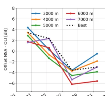
Gaseous attenuation is not accounted for because both sites are expected to be, on average, equally affected. The cutoff altitude has to be high enough to avoid local impacts (e.g., due to pollution Maahn et al., 2017) and biases due to in-dividual frontal systems but low enough to get a sufficient number of observations. For the latter, we have to consider the low height of the Arctic tropopause in winter. To identify the best cutoff height for every three month period, we apply different cutoff altitudes from 3000 to 7000 m to the data set and compare two quality control measures. First, we com-pare the vertical profiles of mean(Ze) for OLI and NSA
be-fore and after relative calibration. Second, we estimate cloud top altitude statistics, which depend strongly on radar sensi-tivity (Protat et al., 2011), using 500 m bins before and after calibration. We choose the cutoff height whose root-mean-square differences after calibration are best based on both methods.
4 Results and discussion
In the following, we apply the three new calibration methods introduced above to the data sets of NSA (Sect. 4.1, Fig. 5) and OLI (Sect. 4.2, Fig. 6) in 2016. In Sect. 4.3, we will com-pare the new methods to the high-altitude reference method. We quantify the calibration quality using the calibration off-setOdefined as follows:
Zetruth=Zmeasurede +O. (2)
To investigate temporal trends, we group the data monthly and estimate the calibration offset for every month sepa-rately. We chose monthly intervals as a compromise be-tween the ability to resolve rapid calibration changes and the need for a sufficient number of liquid cloud observations with varying microphysical properties. The only exception is June 2016 because the radar configuration was changed at OLI on 16 June 2016 (see Table 1), potentially affecting radar calibration. Therefore, the June data set contains only observations from the first half of June and the remaining ob-servations are combined with the July obob-servations. Due to instrument issues in the second half of June, this affects only a few observations.
4.1 Calibration of North Slope of Alaska (NSA) data For NSA, the monthly Ze–γ relationships follow a
sinusoidal-type curve similar to the box model (Fig. 5a), indicating that the phase classification is correctly identi-fying liquid clouds. This is also supported by the fact that all but one month (April 2016) feature W <0.2 m s−1 for Ze<−25 dBz, as expected for liquid clouds without ice
(Fig. 5e). Also, most monthly LWP–max(Ze) relationships
(Fig. 5i) have a similar shape and align within a couple of dB. For theZe–γ relationship, most monthly relationships have
Zeγ=0values between−20 to−17 dBz, but there are a couple
of outliers. The monthlyZe–γ relationships that are shifted
towards smaller (e.g., December 2016) or larger values (e.g., July 2016) show a similar shift for theZe–Wrelationship,
in-dicating that both methods are consistent. The shift in the cor-responding LWP–max(Ze) relationships is smaller, but the
December and July relationships are still below and above the mean relationship, respectively (Fig. 5i). As discussed above, this could be related not only to a change in radar cal-ibration but also to a change in the dominating microphysi-cal conditions. We estimate the microphysi-calibration offsetsOγ=0and OW=0.25 from Zγe=0 and ZWe =0.25, respectively, following
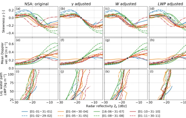
differ-Figure 5.Observed reflectivityZe– skewnessγ(a),Ze– mean Doppler velocityW(e), and liquid water path LWP–max(Ze)(i)relationships
for the North Slope of Alaska (NSA). The data have been calibration-corrected using theγ method (second column), theWmethod (third column), and the LWP method (fourth column). The colored lines indicate the various calibration periods of 2016. The black stars (rows 1 and 2) show the reference point used for calibration; the dotted black line (row 3) is the reference LWP–max(Ze) relationship obtained from
the mean of the monthly relationships weighted by the number of observations.
Figure 6.As in Fig. 5 but for Oliktok Point (OLI).
ences are smallest in summer when the number of observa-tions is largest (corresponding to the number of reflectivity observations in the two bins adjacent toZeγ=0andZW=0.25e ,
Fig. 7c). Because the methods require a sufficient number of drizzling liquid clouds, we expect that the accuracy of
the calibration estimate is reduced in winter. The sensitiv-ity study (Sect. 3.1.1) revealed that higherNtot
concentra-tions for fixed LWC could lead to higherZγe=0andZW=0.25e
and leads to enhancedNtot values, the increasedOγ=0and
OW=0.25 could be related to a change in Ntot values.
Be-sides this potentially seasonal impact, we cannot identify any trends for NSA. The yearly mean values of 1.8 and 0.1 dB for Oγ=0andOW=0.25, respectively, indicate a slight posi-tive calibration offset for NSA. Given the uncertainties, this agrees with Kollias et al. (2019), who estimated KAZR’sO to be around 3 dB at NSA by using CloudSat observations.
We did not estimate a reference LWP–max(Ze)
relation-ship from a model, but given that the KAZR’s calibration at NSA is – according to the γ andW methods – stable and accurate within 2 dB, we can use the LWP–max(Ze)
re-lationship at NSA as a reference. We obtain the reference by taking the mean of the monthly LWP–max(Ze)
relation-ships weighted by the number of observations. Based on the average of the yearly meanOγ=0andOW=0.25 values (1.8 and 0.1 dB, respectively), we apply anOvalue of 1 dB (see Table 4). This allows us to estimate monthly OLWP values from the mean difference between the reference and the cor-responding monthly relationship (Fig. 7a, Table 3). We de-cided to weight the mean difference by the number of obser-vations in each LWP bin because the seasonality of the LWP distribution is high and there are only few observations for higher LWP values in winter. Bins with fewer than 100 ob-servations are skipped. Obviously, this is of limited use for determining an absolute calibration at NSA, but it allows us to compare the variability ofOLWPwithOγ=0andOW=0.25. OLWPvaries between−1.6 and 1.9 dB with a standard devi-ation of 1.1 dB, which is a∼50 % reduction in comparison toOγ=0(2.5 dB) andOW=0.25(2.0 dB). Because it is highly unlikely that a variation in the realOwould compensate for the variability ofOLWPbut not the variability ofOγ=0and OW=0.25, we conclude that the LWP–max(Ze) method is the
most stable method. The uncertainty of the LWP method is probably half of the two drizzle onset methods (i.e., 1.5 dB). Another way to compare the accuracy is to compare the Ze-based relationships after correcting using the various
cal-ibration methods. Of course, the variability ofZγe=0is zero
when applying Oγ=0 (Fig. 5b) and the same applies toW (Fig. 5g) and LWP (Fig. 5l). Also, OW=0.25 leads to a re-duction of the variability ofZγe=0relationship and vice versa
(Fig. 5c, f). This shows the consistency of both methods but is also related to the fact that theZeγ=0 andZW=0.25e
refer-ence values are close, thus both methods use similar sub-data sets. When applying, e.g., OLWP to the Ze–γ relationship
(Fig. 5d), the variability ofZeγ=0is not reduced; the inverse
operation (applying Zγe=0 to LWP–max(Ze) relation) even
enhances the variability (Fig. 5j). This indicates that the vari-ability ofOγ=0,OW=0.25 andOLWP is dominated by their intrinsic variability and not by real changes inO. This is an-other indication thatOat NSA was very stable in 2016.
4.2 Calibration of Oliktok Point (OLI) data
For OLI, the relationships align less well than for NSA. Even though most Ze–γ relationships show a
quasi-sinusoidal shape,Zγe=0varies between approximately−28
and −12 dBz (Fig. 6a). This is confirmed by the spread of ZW=0.25e (Fig. 6e) and the LWP–max(Ze) relationships
(Fig. 6i), which vary consistently with the Ze–γ
relation-ships. The correspondingOγ=0,OW=0.25 andOLWP (with the latter estimated using NSA as a reference, Table 4) val-ues vary between−6.9 and 11.0 dB (dotted lines Fig. 7b). There is no reason why the intrinsic variability of the rela-tionships at OLI should be that much higher than at NSA. We conclude that the KAZR at OLI was not properly cali-brated, withO likely strongly changing with time. We note that some monthly relationships look different even after ap-plying Oγ=0, OW=0.25 and OLWP (estimated using NSA as a reference, Table 4). Even after applying a calibration correction (Fig. 6b, g, l), the spread of the relationships is larger than for NSA. Some months have a drastically reduced amplitude of theZe–γ relationship. Further, many months
featureW >0.25 m s−1also for Ze<−20 dBz. Lastly, the
LWP–max(Ze) relationship is much more curved than the
reference relationship in some months. This indicates that the phase classification was not working properly and the data set also contains nonliquid clouds. The phase classifi-cation by Shupe (2007) depends on absoluteZevalues, e.g.,
by assuming that – under certain conditions – clouds are mixed-phase forZe>−17 dBz. Consequently, a large
pos-itive calibration offsetOmight result in mixed-phase and ice clouds being falsely classified as liquid clouds because their Ze value is underestimated. Mixed-phase and ice clouds,
however, have different and probably more variableZe–γ,
Ze–W, and LWP–max(Ze)relationships. A simple solution
would be to constrain the data set to cases with a tempera-ture larger than 0◦C, but this is not feasible for Arctic sites because few observations would remain. Instead, we run the classification by Shupe (2007) assuming different calibration offsetsOphaseclassfrom−6 to+10 dBz (with 2 dB steps) and estimate the relationships for every assumed offset. Note that Ophaseclassimpacts only which data points are selected based on the phase classification, and we do not modify the Ze
values themselves for obtainingZeγ=0,ZWe =0.25 and the
ref-erence LWP–max(Ze) relationship. To obtain a phase
clas-sification consistent with the calibration offset, we choose the run with the smallest difference betweenOphaseclass and Oγ=0 (or OW=0.25,OLWP). Typically, the smallest differ-ence is less than the 2 dB step size ofOphaseclass. After ac-counting forOphaseclass, the magnitudes of the Ze–γ
rela-tionships are more similar (Fig. 8b), theW for smallZe
val-ues is reduced (Fig. 8g), and the LWP–max(Ze)relationships
Table 3.Estimated offsets for NSA and OLI using the three calibration techniques for NSA and OLI. Our best estimate is to use a constant offset of 1 dB for NSA and to useOLWPfor OLI. A positiveOvalue means theZevalue reported by the radar is too low (Eq. 2).
NSA OLI
Time Oγ=0[dB] OW=0.25[dB] OLWP[dB] Oγ=0[dB] OW=0.25[dB] OLWP[dB]
2016-01-01–2016-01-31 2.3 −1.4 0.8 9.6 7.9 7.9 2016-02-01–2016-02-29 0.2 −0.9 0.4 9.5 7.4 3.7 2016-03-01–2016-03-31 0.2 −0.8 −0.5 11.7 11.1 6.3 2016-04-01–2016-04-30 4.5 3.7 0.6 9.7 6.0 2.7 2016-05-01–2016-05-31 2.2 −1.0 1.5 4.3 3.4 2.7 2016-06-01–2016-06-15 1.1 −1.4 −0.5 7.1 0.9 1.1 2016-06-16–2016-07-31 −2.8 −2.8 0.3 -5.4 −7.2 −4.4 2016-08-01–2016-08-31 1.0 1.4 0.9 −3.5 −3.1 −2.1 2016-09-01–2016-09-30 0.8 1.4 3.0 −4.3 −4.6 −2.3 2016-10-01–2016-10-31 2.8 0.5 1.4 −0.1 −1.6 1.1 2016-11-01–2016-11-30 2.5 −1.0 −1.2 1.3 1.5 −2.0 2016-12-01–2016-12-31 7.2 3.4 1.6 4.3 −3.4 1.9 Estimated uncertainty ±3 ±3 ±1.5 ±3 ±3 ±1.5
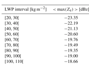
Table 4. Reference LWP–max(Ze) relationship obtained at NSA
using the mean of monthly LWP–max(Ze) relationships weighted
by the number of observations. Note that the meanO was likely around 1±1 dB for NSA, and the reported values in this table are corrected accordingly.
LWP interval [kg m−2] <max(Ze) >[dBz]
[20, 30[ −23.35 [30, 40[ −22.19 [40, 50[ −21.13 [50, 60[ −20.60 [60, 70[ −19.76 [70, 80[ −19.49 [80, 90[ −19.35 [90, 100[ −19.00 [100, 110[ −18.66 [110, 120[ −18.40
makes them more similar to NSA. This indicates that nonliq-uid clouds have been successfully removed from the data set by accounting for Ophaseclass. Interestingly, the differences between O with and without accounting forOphaseclass are often smaller than 2 dB (Fig. 7b). This suggests that the meth-ods are more robust than expected and can provide meaning-ful calibration estimates even if the liquid cloud data sets are contaminated by nonliquid clouds.
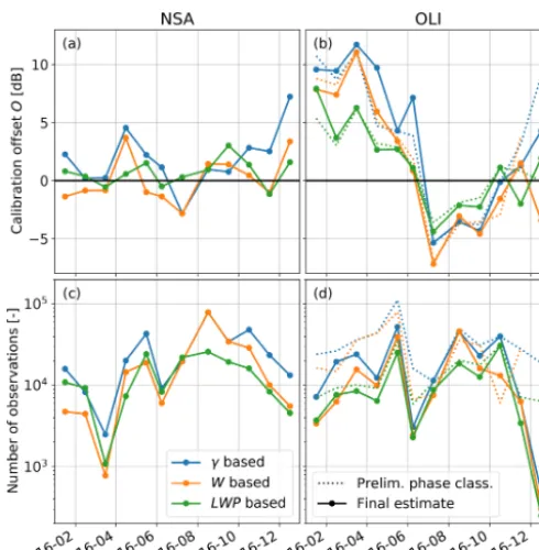
When analyzingOvalues for OLI, the decrease from June to July 2016 stands out. Even though the decrease magni-tude varies between−5.6 and −12.5 dB, all methods show this decrease (Fig. 7b, Table 3), and a similar change was re-ported by Kollias et al. (2019). Based on discussions with the DOE ARM program, the decrease coincides with a change in the KAZR radar configuration (including the calibration
con-stant) on 16 June 2016, though the details of the change are unclear. To find out more about this decrease, we also an-alyze collocated KaSACR measurements. Even though the KaSACR data set size was not sufficient to apply the new calibration methods, we can compare KaSACR and KAZR Ze measurements directly for the two weeks before and
af-ter the step on 16 June 2016. This comparison shows a de-crease in the difference between both radars of 7.5 dB (not shown). Because we have no indication for a simultaneous change in the KaSACR’s configuration or calibration, we at-tribute this change to the KAZR confirming the step identi-fied by the liquid cloud methods. The fact that the relative dif-ference between KAZR and KaSACR was almost zero after 16 June 2016 indicates that the change of the KAZR’s con-figuration was made on purpose to make the measurements of both radars match. After June, all liquid cloud methods show a gradual increase inOwith time. Except for Decem-ber 2016, where fewer than 1000 observations are available, the agreement of the various methods is high, which indi-cates that the gradual trend is likely related to the radar and not to the intrinsic variability of the liquid cloud methods. The gradual trend could indicate hardware problems or a de-pendence ofOon the ambient temperature. The latter could also explain the gradual decrease in O before June 2016. Even though all methods agree about the sign of the trend in spring,Ois higher for theγ- andW-based methods than for the LWP method, which is similar to our results for NSA. Therefore, the higherOγ=0 and OW=0.25 values could be related to Arctic haze, which apparently has a larger impact onZeγ=0andZeW=0.25than the LWP–max(Ze) relationship.
Figure 7.Calibration offsetsO(a, b)and number of used observa-tions(c, d)for NSA(a, c)and OLI(b, d). For OLI, the dotted lines show the preliminary results without modifying the phase classifi-cation withOphaseclass.
The median difference between Oγ=0 and OW=0.25 is very similar for OLI and NSA (1.6 and 1.7 dB, respectively), which could indicate a systematic bias between our box-model-based estimations ofZeγ=0andZeW=0.25. The fact that
the meanOγ=0value of 1.8 dB for NSA for 2016 is closest to the 3 dB estimate of Kollias et al. (2019) might suggest thatZeγ=0is closer to reality thanZeW=0.25.
4.3 Relative calibration of North Slope of Alaska (NSA) and Oliktok Point (OLI) data
The high-altitude calibration method only allows a relative calibration, which we analyze in Fig. 9 for NSA and OLI. We found that individual events can bias the statistics when applying the high-altitude calibration method to monthly pe-riods; therefore, we applied the methods to intervals of three months with the bin threshold of 1 July 2016 shifted to 16 June 2016. The standard deviation between the differ-ent cutoff heights varies between 0.9 and 2.3 dB, which is probably a good estimate for the uncertainty of the high-altitude calibration method. Assuming that the NSA calibra-tion was stable, the relative comparison reveals the decrease inO at OLI on 16 June 2016. When using the best cutoff altitudes, the decrease is estimated to be−5.9 dB, which is – given the different time intervals used for estimatingO – in good agreement with the estimate based on the KaSACR– KAZR comparison (−7.5 dB) and the LWP-based method (−5.6 dB).
A comparison of relative calibration with the high-altitude cloud method and the new methods (Sects. 3.1, 3.2) is pre-sented in Fig. 10. This requires deriving a relative calibration fromOγ=0,OW=0.25, andOLWP by subtracting OLI from NSA and averaging the monthlyO estimates to 3-monthly values. While the combination of both calibrations generally combines the uncertainties of both estimates, some poten-tial error sources cancel out. This is particularly true for any constant or seasonal biases of estimatingZeγ=0,ZeW=0.25, or
the reference LWP–max(Ze) relationship. Given the
uncer-tainties, there is excellent agreement (difference<3 dB) be-tween the high-altitude and liquid cloud methods for April to December 2016 showing the general feasibility of the liq-uid cloud methods. For the winter period (January–March), the agreement is worse, which is likely related to the less robust statistics due to the reduced number of liquid clouds. Moreover, the data sets used for the high-altitude method and the liquid cloud method are not necessarily obtained at the same time even though they are averaged to the same in-tervals. This would require the high-altitude ice clouds and the liquid clouds to always occur at the same time, which is not the case. In particular, whenO is shifting quickly, such a temporal mismatch can contribute to the observed differ-ences between the methods. Even though the difference be-tween the LWP-based method and the high-altitude clouds method can be up to 2.7 dB in late 2016, the mean difference is lower (0.9 dB) than for theγ-based (2.0 dB) andW-based (1.6 dB) methods. This confirms our previous conclusion that the LWP-based method has the smallest intrinsic variability and likely works best for estimatingOin the Arctic.
5 Summary and conclusions
In this study, we investigate the potential for using the im-print of liquid cloud processes on DSDs for radar calibration. Specifically, we investigate the relationships of radar reflec-tivelyZeto the skewness of the radar Doppler spectrumγ
and to the mean Doppler velocityW. Moreover, we use the relationship between the maximumZe value in the column
(max(Ze)) and the liquid water path LWP measured by a
mi-crowave radiometer (MWR). These methods close an impor-tant gap in our ability to monitor and assess radar calibration. The fact that we focus only on drizzle onset for theZe–γ
andZe–Wrelationships allows us to use a box model
(Hoff-mann et al., 2017) coupled to the PAMTRA2 radar simu-lator (Maahn et al., 2015) to determine the dependency of the relationship on the initial DSD and random effects. De-pending on initial cloud microphysical conditions and, to a lesser extent, random effects, we determine typical rela-tionships for γ and W as a function of Ze. We find that
compensation and saturation effects reduce the variability of theZe–γ andZe–W relations, which allows us to
Figure 8.As in Fig. 6 but considering a calibration offset for the phase classification.
Figure 9.Comparison relative calibration offsets NSA–OLI for dif-ferent cutoff heights (colored lines). The best estimate (see text) is highlighted in black.
smallest forZeγ=0= −17.6±3 dBz when cloud droplets and
drizzle contribute to reflectivity equally, i.e.,γ=0. ForW, we identify the smallest variability forW=0.25 m s−1and ZWe =0.25= −16.6±3 dBz. Because we cannot quantify feed-back effects of clouds and their environment on the LWP– max(Ze) relationship with a box model, we do not use a
model to obtain a reference relationship. Instead, we use the approach for relative calibration between two radars.
Applying the methods to radar observations of low-level Arctic liquid clouds at the ARM North Slope of Alaska (NSA) and Oliktok Point (OLI) sites, we identify medianZe–
γ,Ze–W, and LWP–max(Ze) relationships. We applied the
methods to monthly intervals to identify rapid changes but
Figure 10.Comparison of relative calibrations NSA–OLI usingγ (Oγ=0, blue line),W(OW=0.25, orange line), and the high-altitude method (green line). All methods have been averaged to the same temporal resolution; the original resolutions are indicated by the dashed lines. For clarity, the lines have been slightly shifted along thexaxis.
obtain a sufficient number of liquid cloud observations (at least 1000 data points for a 15 s temporal resolution). For NSA, the observed relationships are in general agreement with the box model simulations and we successfully iden-tify the referenceZe values forγ=0 (−17.3±3 dBz) and
W=0.25 (−16.3±3 dBz). We use the difference between measured and modeledZereference values for assessing the
relatively stable andO is on average around 1 dB (Fig. 7a). The good calibration of the NSA KAZR motivated us to use the LWP–max(Ze) relationship at NSA as a reference for
absolute calibration. The variability of the estimatedOLWP is smaller than for Oγ=0 andOW=0.25, indicating that the LWP-based method has an uncertainty of about 1.5 dB and is less impacted by microphysical and dynamical conditions. The difference between the methods is largest for the winter months (Fig. 7a), indicating that the lower number of liq-uid clouds might limit the quality of theOestimation. Also, the phase classification algorithm employed might struggle in winter to remove all mixed-phase clouds from the data set as required.
For OLI, we identify serious problems with maintaining an accurate radar calibration. Most remarkably, we find that O decreased 5 to 7 dB in June 2016 (Fig. 7b), which was likely related to a change in radar configuration even though the details cannot be reconstructed. Further, we identify a slowly decreasing and increasing trend of O in spring and fall, respectively, of 2016. Similar to NSA, the agreement between the liquid-cloud-based methods is reduced during winter, indicating that a sufficient number of liquid cloud samples is required for the method to work properly. Despite this, theZe–γ,Ze–W, and LWP–max(Ze) relationships for
OLI are consistent after application of a calibration correc-tion (Fig. 6b, g, l). This indicates the ability of the methods to correct also for largerO values as long as the calibration offset is considered during the phase classification (Shupe, 2007) for identifying liquid clouds. The LWP-based method matches the high-altitude cloud reference method best. Con-sidering the error margins, our results are in excellent agree-ment with Kollias et al. (2019). By applying the CloudSat method by Protat et al. (2011), they found a similar drop for OLI and a 3 dB offset for NSA.
In summary, we find that liquid cloud microphysical pro-cesses can be used for radar calibration in the Arctic. The Ze–γ,Ze–W, and LWP–max(Ze) relationships contain
valu-able information that can be used to determine the cloud radar calibration offset O. Due to the effect of turbulence on radar observations, theγ-based method likely works best for stratiform clouds, which are typically not that turbulent. In comparison to other calibration methods for cloud radars, the new methods have several advantages. Most importantly, no dedicated field campaigns are required and the methods can be easily applied to past data sets. In comparison to the method by Protat et al. (2011), the liquid cloud microphysical processes methods can be applied to shorter time intervals, which better enables the detection of sudden changes. Also, our methods do not depend on CloudSat, which is likely close to the end of its lifetime. Further, the method can be – with limited accuracy in winter – applied to year-round ob-servations even at high latitudes because liquid clouds occur throughout the year. Theγ- and W-based methods require supporting instrumentation (microwave radiometer, lidar, ra-diosonde observations) only for the identification of liquid
clouds. If the presence of ice and mixed-phase clouds can be ruled out by other means (e.g., at subtropical or tropical sites), application of the method is possible without any ad-ditional instrumentation. The LWP-based method requires a collocated MWR that has to be calibrated carefully using an offset correction during clear-sky periods. While we found the LWP-based method to work best, the question of whether Zeγ=0orZWe =0.25 is the second-best method for calibration
is still open. The box model indicates a larger stability for Zeγ=0, but the variability of observed ZeW=0.25 is lower at
NSA. Assuming the NSA KAZR calibration was stable, this would indicate that ZWe =0.25 is slightly better suited. Yet, ZeW=0.25 is more easily affected by biases, e.g., due to per-sistent vertical air motions related to orography. These biases could be an explanation for the small 1.6 to 1.7 dB offset be-tween the Zeγ=0- and ZeW=0.25-based calibration estimates.
Instead,γ is less affected by biases, but the observations are noisier, require a high temporal resolution, and most stan-dard radar products do not include γ. Likely, it is best to apply all three methods and use the agreement between the methods as an indicator for the quality of the calibration off-set estimate. With respect to the calibration offoff-setOfor OLI and NSA in 2016, we recommend using the results of the LWP–max(Ze) method for OLI (Fig. 7b, Table 3) and using
an offset of+1 dB for NSA.
Further research is needed to reduce the uncertainty of the methods and to assess the dependence of the referenceZe
values on climatological and environmental conditions like the availability of cloud condensation nuclei. The reference Zevalues and relationships need to be carefully reevaluated
when applying the method to radar observations from other regions. This also applies to the LWP–max(Ze) relationship
where we used the relationship obtained at NSA as a refer-ence. However, it is not clear whether this relationship is ap-plicable to other sites or whether it is valid only at the North Slope of Alaska. Sites with a radar with stable calibration off-sets could be used to assess the seasonality of the used refer-ence relationships over multiple years. Further, an extension of the method to mixed-phase and ice clouds would be de-sirable, but the greater variability of ice particles shapes, fall velocities, and radar backscattering cross sections makes this even more challenging than for liquid clouds. Even though the method has been developed forKa-band cloud radars, it