Computer Vision Metrics

(1)

Shelve in Graphics/General User level: Beginning–Advanced

Computer Vision Metrics

Computer Vision Metrics: Survey, Taxonomy, and Analysis provides a technical tour through computer vision, with a survey of nearly 100 types of local, regional, and global feature descriptors, blending history of the field with state-of-the-art analysis of contemporary methods, rather than just another how-to book with source code shortcuts and performance analysis. Observations are provided to develop intuition behind the methods and mathematics, interesting questions are raised for future research rather than providing all the answers, and a Vision Taxonomy is suggested to draw a conceptual map of the field. Extensive illustrations are included, with over 540 references to the literature in the comprehensive bibliography to dig deeper.

Computer Vision Metrics explores the key questions behind the design and mathematics of computer vision metrics and feature descriptors, providing a comprehensive survey and taxonomy of what methods are used, with analysis and observations about why the methods work. Several 3D depth sensing methods are surveyed including MVS, stereo, and structured light.

This work focuses on a slice through the field from the view of feature description metrics, or how to describe, compute, and design the macro-features and micro-features that make up larger objects in images. The focus is on the pixel-side of the vision pipeline, with a light introduction to the back-end training, classification, machine learning, and matching stages.

Computer Vision Metrics is written for engineers, scientists, and academic researchers in areas including video analytics, scene understanding, machine vision, face recognition, gesture recognition, pattern recognition, general object analysis, media processing, and computational photography.

What You’ll Learn:

• Current status, brief history, and future directions for computer vision metrics • Taxonomy of local binary, gradient & other spectra, shape features,

and basis spaces

• Overview of 2D image sensing, 3D depth sensing, and image preprocessing • Vision pipeline optimization methods for computer vision applications • Characterization of ten OpenCV detectors using synthetic feature alphabets

9 781430 259299 5 3 9 9 9 ISBN 978-1-4302-5929-9

(2)

For your convenience Apress has placed some of the front

matter material after the index. Please use the Bookmarks

and Contents at a Glance links to access them.

(3)

Contents at a Glance

About the Author ��

�xxvii

Acknowledgments ��

xxix

Introduction ��

xxxi

Chapter 1: Image Capture and Representation

■

��

1 Chapter 2: Image Pre-Processing

■

��

39 Chapter 3: Global and Regional Features

■

��

85 Chapter 4: Local Feature Design Concepts, Classification,

■

and Learning ��

131 Chapter 5: Taxonomy of Feature Description Attributes

■

��

191 Chapter 6: Interest Point Detector and Feature

■

Descriptor Survey ��

217 Chapter 7: Ground Truth Data, Content, Metrics, and Analysis

■

��

283 Chapter 8: Vision Pipelines and Optimizations

■

��

313 Appendix A: Synthetic Feature Analysis

■

��

365 Appendix B: Survey of Ground Truth Datasets

■

��

401 Appendix C: Imaging and Computer Vision Resources

■

��

411 Appendix D: Extended SDM Metrics

■

��

419 Bibliography

■

��

437

(4)

Introduction

Dirt. This is a jar of dirt.

Yes.

. . . Is the jar of dirt going to help?

If you don’t want it, give it back.

—

Pirates Of The Carribean

, Jack Sparrow and Tia Dalma

This work focuses on a slice through the field - Computer Vision Metrics – from the view of feature description metrics, or how to describe, compute and design the macro-features and micro-features that make up larger objects in images. The focus is on the pixel-side of the vision pipeline, rather than the back-end training, classification, machine learning and matching stages. This book is suitable for reference, higher-level courses, and self-directed study in computer vision. The book is aimed at someone already familiar with computer vision and image processing; however, even those new to the field will find good introductions to the key concepts at a high level, via the ample illustrations and summary tables.

I view computer vision as a mathematical artform and its researchers and

practitioners as artists. So, this book is more like a tour through an art gallery rather than a technical or scientific treatise. Observations are provided, interesting questions are raised, a vision taxonomy is suggested to draw a conceptual map of the field, and references are provided to dig deeper. This book is like an attempt to draw a map of the world centered around feature metrics, inaccurate and fuzzy as the map may be, with the hope that others will be inspired to expand the level of detail in their own way, better than what I, or even a few people, can accomplish alone. If I could have found a similar book covering this particular slice of subject matter, I would not have taken on the project to write this book.

What is not in the Book

(5)

since the bibliography references cover these matters quite well: for example, machine learning, training and classification methods are only lightly introduced, since the focus here is on the feature metrics.

In summary, this book is about the feature metrics, showing “‘what”’ methods practitioners are using, with detailed observations and analysis of “‘why”’ those methods work, with a bias towards raising questions via observations rather than providing too many answers. I like the questions best because good questions lead to many good answers, and each answer is often pregnant with more good questions...

This book is aimed at a survey level, with a taxonomy and analysis, so no detailed examples of individual use-cases or horse races between methods are included. However, much detail is provided in over 540+ bibliographic references to dig deeper into practical matters. Additionally, some “‘how-to”’ and “‘hands-on”’ resources are provided in Appendix C. And a little ‘perfunctory’ source code accompanying parts of this book is available online, for Appendix A covering the interest point detector evaluations for the synthetic interest point alphabets introduced in Chapter 7; and in Appendix D for extended SDM metrics covered in Chapter 3.

What is in the Book

Specifically, Chapter 1 provides preamble on 2d image formation and 3d depth imaging, and Chapter 2 promotes intelligent image pre-processing to enhance feature description. Chapters 3 through 6 form the core discussion on feature description, with an emphasis on local features. Global and regional metrics are covered in Chapter 3, feature descriptor concepts in Chapter 4, a vision taxonomy is suggested in Chapter 5, and local feature description is covered in Chapter 6. Ground truth data is covered in Chapter 7, and Chapter 8 discusses hypothetical vision pipelines and hypothetical optimizations from an engineering perspective, as a set of exercises to tie vision concepts together into real systems (coursework assignments can be designed to implement and improve the hypothetical examples in Chapter 8). A set of synthetic interest point alphabets is developed in Chapter 7, and ten common detectors are run against those alphabets, with the results provided in Appendix A. It is difficult to cleanly partition all topics in image processing and computer vision, so there is some overlap in the chapters. Also, there are many hybrids used in practice, so there’s inevitable overlap in the Chapter 5 vision taxonomy, and creativity always arrives on the horizon to find new and unexpected ways of using old methods. However, the taxonomy is a starting point and helped to guide the organization of the book.

(6)

Scope

For brevity’s sake, I exclude a deep treatment of selected topics not directly related to the computer vision metrics themselves; this is an unusual approach, since computer vision discussions typically include a wider range of topics. Specifically, the topics not covered deeply here include statistical and machine learning, classification and training, feature database construction and optimization, and searching and sorting. Bibliography references are provided instead. Distance functions are discussed, since they are directly linked to the feature metric. (A future edition of this book may contain a deep dive into the statistical and machine learning side of computer vision, but not now.)

Terminology Caveat

Sometimes terminology in the literature does not agree when describing similar concepts. So in some cases, terminology is adopted in this work that is not standardized across independent research communities. In fact, some new and nonstandard terminology may be introduced here, possibly because the author is unaware of better existing terminology (perhaps some of the terminology introduced in this work will become standardized). Terminology divergence is most pronounced with regard to mathematical topics like clustering, regression, group distance, and error minimization, as well as for computer vision topics like keypoints, interest points, anchor points, and the like. The author recognizes that one is reluctant to change terminology, since so many concepts are learned based on the terminology. I recall a friend of mine, Homer Mead, chief engineer for the lunar rover and AWACS radar at Boeing, who sub-consciously refused to convert from using the older term condenser to use the newer term capacitor.

Inspiration comes from several sources, mostly the opportunity of pioneering: there is always some lack of clarity, structure and organization in any new field as the boundaries expand, so in this vast field the opportunity to explore is compelling: to map out structure and pathways of knowledge that others may follow to find new fields of study, create better markers along the way, and extend the pathways farther.

(7)

Western Systems and later at Applied Precision, asked me to analyze the View-PRB fixed-function hardware unit for pattern recognition to use for automatic wafer probing (in case we needed to build something like it ourselves) to locate patterns on wafers and align the machine for probing. Correlation was used for pattern matching, with a scale-space search method we termed “super-pixels.” The matching rate was four 32x32 patches per second over NTSC with sub-pixel accuracy, and I computed position, rotation, and offsets to align the wafer prober stage to prepare for wafer probing; we called this auto-align. I designed a pattern recognition servo system to locate the patterns with rotational accuracy of a few micro-radians, and positional accuracy of a fraction of a micron. In the later 1980s, I went to work for Mentor Graphics, and after several years I left the corporate R&D group reporting to the president Gerry Langeler to start a company, Krig Research, to focus on computer vision and imaging for high-end military and research customers based on expensive and now extinct workstations (SGI, Apollo, Sun… gone, all gone now…), and I have stayed interested ever since. Many things have changed in our industry; the software seems to all be free, and the hardware or SOC is almost free as well, so I am not sure how anyone can make any money at this anymore.

More recently, others have also provided inspiration. Thanks to Paul Rosin for synthetic images and organizational ideas. Thanks to Yann LeCun for providing key references into deep learning and convolutional networks, and thanks to Shree Nayar for permission to use a few images, and continuing to provide the computer vision community with inspiration via the Cave Research projects. And thanks to Luciano Oviedo for vast coverage of industry activity and strategy about where it is all going, and lively discussions.

Others, too many to list, have also added to my journey. And even though the

conversations have sometimes been brief, or even virtual via email or SKYPE in many cases, the influence of their work and thinking has remained, so special thanks are due to several people who have provided comments to the manuscript or book outline, contributed images, or just plain inspiration they may not realize. Thank you to Rahul Suthankar, Alexandre Alahi for use of images and discussions; Steve Seitz, Bryan Russel, Liefeng Bo, and Xiaofeng Ren for deep-dive discussions about RGB-D computer vision and other research topics; Gutemberg Guerra-filho, Harsha Viswana, Dale Hitt, Joshua Gleason, Noah Snavely, Daniel Scharstein, Thomas Salmon, Richard Baraniuk, Carl Vodrick, Hervé Jégou, and Andrew Richardson; and also thanks for many interesting discussions on computer vision topics with several folks at Intel including Ofri Weschler, Hong Jiang, Andy Kuzma, Michael Jeronimo, Eli Turiel, and many others whom I have failed to mention.

Summary

In summary, my goal is to survey the methods people are using for feature description— the key metrics generated—and make it easier for anyone to understand the methods in practice, and how to evaluate the methods using the vision taxonomy and robustness criteria to get the results they are looking for, and find areas for extending the state of the art. And after hearing all the feedback from the first version of this work, I hope to create a second version that is even better.

(8)

Image Capture

and Representation

“The changing of bodies into light, and light into bodies, is very

conformable to the course of Nature, which seems delighted with

transmutations.”

—Isaac Newton

Computer vision starts with images. This chapter surveys a range of topics dealing with capturing, processing, and representing images, including computational imaging, 2D imaging, and 3D depth imaging methods, sensor processing, depth-field processing for stereo and monocular multi-view stereo, and surface reconstruction. A high-level overview of selected topics is provided, with references for the interested reader to dig deeper. Readers with a strong background in the area of 2D and 3D imaging may benefit from a light reading of this chapter.

Image Sensor Technology

This section provides a basic overview of image sensor technology as a basis for understanding how images are formed and for developing effective strategies for image sensor processing to optimize the image quality for computer vision.

(9)

Image sensors are designed to reach specific design goals with different applications in mind, providing varying levels of sensitivity and quality. Consult the manufacturer’s information to get familiar with each sensor. For example, the size and material composition of each photo-diode sensor cell element is optimized for a given semiconductor manufacturing process so as to achieve the best tradeoff between silicon die area and dynamic response for light intensity and color detection.

For computer vision, the effects of sampling theory are relevant—for example, the Nyquist frequency applied to pixel coverage of the target scene. The sensor resolution and optics together must provide adequate resolution for each pixel to image the features of interest, so it follows that a feature of interest should be imaged or sampled at two times the minimum size of the smallest pixels of importance to the feature. Of course, 2x oversampling is just a minimum target for accuracy; in practice, single pixel wide features are not easily resolved.

For best results, the camera system should be calibrated for a given application to determine the sensor noise and dynamic range for pixel bit depth under different lighting and distance situations. Appropriate sensor processing methods should be developed to deal with the noise and nonlinear response of the sensor for any color channel, to detect and correct dead pixels, and to handle modeling of geometric distortion. If you devise a simple calibration method using a test pattern with fine and coarse gradations of gray scale, color, and pixel size of features, you can look at the results. In Chapter 2, we survey a range of image processing methods applicable to sensor processing. But let’s begin by surveying the sensor materials.

Sensor Materials

Silicon-based image sensors are most common, although other materials such as gallium (Ga) are used in industrial and military applications to cover longer IR wavelengths than silicon can reach. Image sensors range in resolution, depending upon the camera used, from a single pixel phototransistor camera, through 1D line scan arrays for industrial applications, to 2D rectangular arrays for common cameras, all the way to spherical arrays for high-resolution imaging. (Sensor configurations and camera configurations are covered later in this chapter.)

Common imaging sensors are made using silicon as CCD, CMOS, BSI, and Foveon methods, as discussed a bit later in this chapter. Silicon image sensors have a nonlinear spectral response curve; the near infrared part of the spectrum is sensed well, while blue, violet, and near UV are sensed less well, as shown in Figure 1-2. Note that the silicon spectral response must be accounted for when reading the raw sensor data and quantizing the data into a digital pixel. Sensor manufacturers make design compensations in this area; however, sensor color response should also be considered when calibrating your camera system and devising the sensor processing methods for your application.

Micro-lenses RGB Color Filters CMOS imager

(10)

Sensor Photo-Diode Cells

One key consideration in image sensoring is the photo-diode size or cell size. A sensor cell using small photo-diodes will not be able to capture as many photons as a large photo-diode. If the cell size is below the wavelength of the visible light to be captured, such as blue light at 400nm, then additional problems must be overcome in the sensor design to correct the image color. Sensor manufacturers take great care to design cells at the optimal size to image all colors equally well (Figure 1-3). In the extreme, small sensors may be more sensitive to noise, owing to a lack of accumulated photons and sensor readout noise. If the photo-diode sensor cells are too large, there is no benefit either, and the die size and cost for silicon go up, providing no advantage. Common commercial sensor devices may have sensor cell sizes of around 1 square micron and larger; each manufacturer is different, however, and tradeoffs are made to reach specific requirements.

(11)

Sensor Configurations: Mosaic, Foveon, BSI

There are various on-chip configurations for multi-spectral sensor design, including mosaics and stacked methods, as shown in Figure 1-4. In a mosaic method, the color filters are arranged in a mosaic pattern above each cell. The Foveon1_{sensor stacking}

method relies on the physics of depth penetration of the color wavelengths into the semiconductor material, where each color penetrates the silicon to a different depth, thereby imaging the separate colors. The overall cell size accommodates all colors, and so separate cells are not needed for each color.

1.00

0.80

0.60

0.40

0.20

0.00

390 440 540

Wavelength (nm)

Sensitivity

RGB color spectral overlap

640 740

490 590 690

Figure 1-3. Primary color assignment to wavelengths. Note that the primary color regions overlap, with green being a good monochrome proxy for all colors

(12)

Back-side-illuminated (BSI) sensor configurations rearrange the sensor wiring on the die to allow for a larger cell area and more photons to be accumulated in each cell. See the Aptina [410] white paper for a comparison of front-side and back-side die circuit arrangement.

The arrangement of sensor cells also affects the color response. For example, Figure 1-5 shows various arrangements of primary color (R, G, B) sensors as well as white (W) sensors together, where W sensors have a clear or neutral color filter. The sensor cell arrangements allow for a range of pixel processing options—for example, combining selected pixels in various configurations of neighboring cells during sensor processing for a pixel formation that optimizes color response or spatial color resolution. In fact, some applications just use the raw sensor data and perform custom processing to increase the resolution or develop alternative color mixes.

Stacked Photo-diodes

R B

G

R filter

B filter G filter

Photo-diode Photo-diode Photo-diode

Figure 1-4. (Left) The Foveon method of stacking RGB cells to absorb different wavelengths at different depths, with all RGB colors at each cell location. (Right) A standard mosaic cell placement with RGB filters above each photo-diode, with filters only allowing the specific wavelengths to pass into each photo-diode

(13)

The overall sensor size and format determines the lens size as well. In general, a larger lens lets in more light, so larger sensors are typically better suited to digital cameras for photography applications. In addition, the cell placement aspect ratio on the die determines pixel geometry—for example, a 4:3 aspect ratio is common for digital cameras while 3:2 is standard for 35mm film. The sensor configuration details are worth understanding so you can devise the best sensor processing and image pre-processing pipelines.

Dynamic Range and Noise

Current state-of-the-art sensors provide at least 8 bits per color cell, and usually are 12 to 14 bits. Sensor cells require area and time to accumulate photons, so smaller cells must be designed carefully to avoid problems. Noise may come from optics, color filters, sensor cells, gain and A/D converters, post-processing, or the compression methods, if used. Sensor readout noise also affects effective resolution, as each pixel cell is read out of the sensor, sent to an A/D converter, and formed into digital lines and columns for conversion into pixels. Better sensors will provide less noise and higher effective bit resolution. A good survey of de-noising is found in the work by Ibenthal [409].

In addition, sensor photon absorption is different for each color, and may be problematic for blue, which can be the hardest color for smaller sensors to image. In some cases, the manufacturer may attempt to provide a simple gamma-curve correction method built into the sensor for each color, which is not recommended. For demanding color applications, consider colorimetric device models and color management (as will be discussed in Chapter 2), or even by characterizing the nonlinearity for each color channel of the sensor and developing a set of simple corrective LUT transforms. (Noise-filtering methods applicable to depth sensing are also covered in Chapter 2.)

Sensor Processing

Sensor processing is required to de-mosaic and assemble the pixels from the sensor array, and also to correct sensing defects. We discuss the basics of sensor processing in this section.

Typically, a dedicated sensor processor is provided in each imaging system, including a fast HW sensor interface, optimized VLIW and SIMD instructions, and dedicated fixed-function hardware blocks to deal with the massively parallel pixel-processing workloads for sensor processing. Usually, sensor processing is transparent, automatic, and set up by the manufacturer of the imaging system, and all images from the sensor are processed the same way. A bypass may exist to provide the raw data that can allow custom sensor processing for applications like digital photography.

De-Mosaicking

Depending on the sensor cell configuration, as shown in Figure 1-5, various

(14)

One of the central challenges of de-mosaicking is pixel interpolation to combine the color channels from nearby cells into a single pixel. Given the geometry of sensor cell placement and the aspect ratio of the cell layout, this is not a trivial problem. A related issue is color cell weighting—for example, how much of each color should be integrated into each RGB pixel. Since the spatial cell resolution in a mosaicked sensor is greater than the final combined RGB pixel resolution, some applications require the raw sensor data to take advantage of all the accuracy and resolution possible, or to perform special processing to either increase the effective pixel resolution or do a better job of spatially accurate color processing and de-mosaicking.

Dead Pixel Correction

A sensor, like an LCD display, may have dead pixels. A vendor may calibrate the sensor at the factory and provide a sensor defect map for the known defects, providing coordinates of those dead pixels for use in corrections in the camera module or driver software. In some cases, adaptive defect correction methods [408] are used on the sensor to monitor the adjacent pixels to actively look for defects and then to correct a range of defect types, such as single pixel defects, column or line defects, and defects such as 2x2 or 3x3 clusters. A camera driver can also provide adaptive defect analysis to look for flaws in real time, and perhaps provide special compensation controls in a camera setup menu.

Color and Lighting Corrections

Color corrections are required to balance the overall color accuracy as well as the white balance. As shown in Figure 1-2, color sensitivity is usually very good in silicon sensors for red and green, but less good for blue, so the opportunity for providing the most accurate color starts with understanding and calibrating the sensor.

Most image sensor processors contain a geometric processor for vignette correction, which manifests as darker illumination at the edges of the image, as shown in Chapter 7 (Figure 7-6). The corrections are based on a geometric warp function, which is calibrated at the factory to match the optics vignette pattern, allowing for a programmable

illumination function to increase illumination toward the edges. For a discussion of image warping methods applicable to vignetting, see reference [490].

Geometric Corrections

(15)

Cameras and Computational Imaging

Many novel camera configurations are making their way into commercial applications using computational imaging methods to synthesize new images from raw sensor data— for example, depth cameras and high dynamic range cameras. As shown in Figure 1-6, a conventional camera system uses a single sensor, lens, and illuminator to create 2D images. However, a computational imaging camera may provide multiple optics, multiple programmable illumination patterns, and multiple sensors, enabling novel applications such as 3D depth sensing and image relighting, taking advantage of the depth

information, mapping the image as a texture onto the depth map, and introducing new light sources and then re-rendering the image in a graphics pipeline. Since computational cameras are beginning to emerge in consumer devices and will become the front end of computer vision pipelines, we survey some of the methods used.

Single Lens Single Flash

Programmable Flash

- Pattern Projectors

- Multi-Flash Computational Imaging

- High Dynamic Range HDR

- High Frame Rates

- 3D Depth Maps

- Focal Plane Refocusing

- Focal Sweep

- Rolling Shutter

- Panorama Stitching

- Image Relighting

2D Sensor

2D Sensor Array Image Enhancements

- Color Enhancements

- Filtering, Contrast

Multi-lens Optics Arrays

- Plenoptic Lens Arrays

- Sphere/Ball Lenses

Figure 1-6. Comparison of computational imaging systems with conventional cameras. (Top) Simple camera model with flash, lens, and imaging device followed by image enhancements like sharpening and color corrections. (Bottom) Computational imaging using programmable flash, optics arrays, and sensor arrays, followed by computational imaging applications

Overview of Computational Imaging

(16)

Single-Pixel Computational Cameras

Single-pixel computational cameras can reconstruct images from a sequence of single photo detector pixel images of the same scene. The field of single-pixel cameras [103, 104] falls into the domain of compressed sensing research, which also has applications outside image processing extending into areas such as analog-to-digital conversion.

As shown in Figure 1-7, a single-pixel camera may use a micro-mirror array or a

digital mirror device (DMD), similar to a diffraction grating. The gratings are arranged in a rectangular micro-mirror grid array, allowing the grid regions to be switched on or off to produce binary grid patterns. The binary patterns are designed as a pseudo-random binary basis set. The resolution of the grid patterns is adjusted by combining patterns from adjacent regions—for example, a grid of 2x2 or 3x3 micro-mirror regions.

Figure 1-7. A single-pixel imaging system where incoming light is reflected through a DMD array of micro-mirrors onto a single photo-diode. The grid locations within the micro-mirror array can be opened or closed to light, as shown here, to create binary patterns, where the white grid squares are reflective and open, and the black grid squares are closed. (Image used by permission, © R. G. Baraniuk, Compressive Sensing Lecture Notes)

A sequence of single-pixel images is taken through a set of pseudo-random micro lens array patterns, then an image is reconstructed from the set. In fact, the number of pattern samples required to reconstruct the image is lower than the Nyquist frequency, since a sparse random sampling approach is used and the random sampling approach has been proven in the research to be mathematically sufficient [103, 104]. The grid basis-set sampling method is directly amenable to image compression, since only a relatively sparse set of patterns and samples are taken. Since the micro-mirror array us es rectangular shapes, the patterns are analogous to a set of HAAR basis functions. (For more information, see Figures 2-20 and 6-22.)

(17)

2D Computational Cameras

Novel configurations of programmable 2D sensor arrays, lenses, and illuminators are being developed into camera systems as computational cameras [424,425,426], with applications ranging from digital photography to military and industrial uses, employing computational imaging methods to enhance the images after the fact. Computational cameras borrow many computational imaging methods from confocal imaging [419] and confocal microscopy [421, 420]—for example, using multiple illumination patterns and multiple focal plane images. They also draw on research from synthetic aperture radar systems [422] developed after World War II to create high-resolution images and 3D depth maps using wide baseline data from a single moving-camera platform. Synthetic apertures using multiple image sensors and optics for overlapping fields of view using wafer-scale integration are also topics of research [419]. We survey here a few computational 2D sensor methods, including high resolution (HR), high dynamic range

(HDR), and high frame rate (HF) cameras.

The current wave of commercial digital megapixel cameras, ranging from around 10 megapixels on up, provide resolution matching or exceeding high-end film used in a 35mm camera [412], so a pixel from an image sensor is comparable in size to a grain of silver on the best resolution film. On the surface, there appears to be little incentive to go for higher resolution for commercial use, since current digital methods have replaced most film applications and film printers already exceed the resolution of the human eye.

(18)

High dynamic range (HDR) cameras [416,417,418] can produce deeper pixels with higher bit resolution and better color channel resolution by taking multiple images of the scene bracketed with different exposure settings and then combining the images. This combination uses a suitable weighting scheme to produce a new image with deeper pixels of a higher bit depth, such as 32 pixels per color channel, providing images that go beyond the capabilities of common commercial CMOS and CCD sensors. HDR methods allow faint light and strong light to be imaged equally well, and can combine faint light and bright light using adaptive local methods to eliminate glare and create more uniform and pleasing image contrast.

(19)

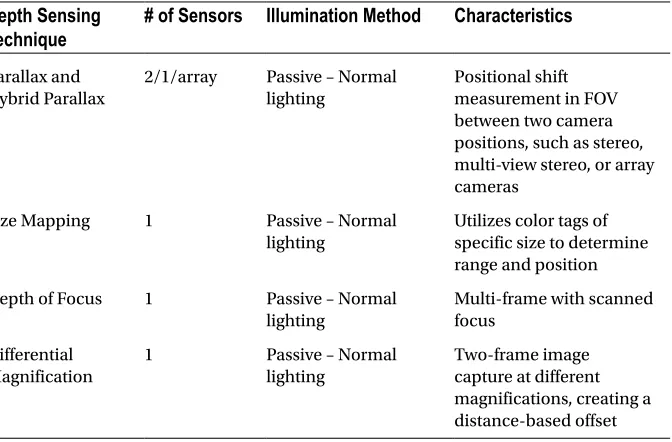
Table 1-1. Selected Methods for Capturing Depth Information

Depth Sensing

Technique

# of Sensors

Illumination Method

Characteristics

Parallax and Hybrid Parallax

2/1/array Passive – Normal lighting

Positional shift measurement in FOV between two camera positions, such as stereo, multi-view stereo, or array cameras

Size Mapping 1 Passive – Normal

lighting

Utilizes color tags of specific size to determine range and position

Depth of Focus 1 Passive – Normal lighting

Multi-frame with scanned focus

Differential Magnification

1 Passive – Normal

lighting

Two-frame image capture at different magnifications, creating a distance-based offset

(continued)

High frame rate (HF) cameras [425] are capable of capturing a rapid succession of images of the scene into a set and combining the set of images using bracketing techniques to change the exposure, flash, focus, white balance, and depth of field.

3D Depth Camera Systems

Using a 3D depth field for computer vision provides an understated advantage for many applications, since computer vision has been concerned in large part with extracting 3D information from 2D images, resulting in a wide range of accuracy and invariance problems. Novel 3D descriptors are being devised for 3D depth field computer vision, and are discussed in Chapter 6.

With depth maps, the scene can easily be segmented into foreground and background to identify and track simple objects. Digital photography applications are incorporating various computer vision methods in 3-space and thereby becoming richer. Using selected regions of a 3D depth map as a mask enables localized image enhancements such as depth-based contrast, sharpening, or other pre-processing methods.

(20)

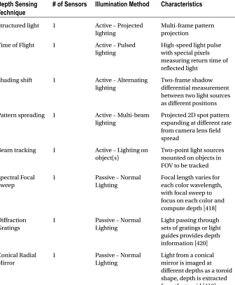
Depth Sensing

Technique

# of Sensors

Illumination Method

Characteristics

Structured light 1 Active – Projected lighting

Multi-frame pattern projection

Time of Flight 1 Active – Pulsed lighting

High-speed light pulse with special pixels measuring return time of reflected light

Shading shift 1 Active – Alternating lighting

Two-frame shadow differential measurement between two light sources as different positions

Pattern spreading 1 Active – Multi-beam lighting

Projected 2D spot pattern expanding at different rate from camera lens field spread

Beam tracking 1 Active – Lighting on object(s)

Two-point light sources mounted on objects in FOV to be tracked

Spectral Focal Sweep

Lighting

Focal length varies for each color wavelength, with focal sweep to focus on each color and compute depth [418]

Diffraction Gratings

Lighting

Light passing through sets of gratings or light guides provides depth information [420]

Conical Radial Mirror

Lighting

Light from a conical mirror is imaged at different depths as a toroid shape, depth is extracted from the toroid [413]

Source: Courtesy of Ken Salsmann Aptina [427], with a few other methods added by the author.

(21)

Depth sensing is not a new field, and is covered very well in several related disciplines with huge industrial applications and financial resources, such as satellite imaging, remote sensing, photogrammetry, and medical imaging. However, the topics involving depth sensing are of growing interest in computer vision with the advent of commercial depth-sensing cameras such as Kinect, enabling graduate students on a budget to experiment with 3D depth maps and point clouds using a mobile phone or PC.

Multi-view stereo (MVS) depth sensing has been used for decades to compute digital elevation maps or DEMs, and digital terrain maps or DTMs, from satellite images using RADAR and LIDAR imaging, and from regional aerial surveys using specially equipped airplanes with high-resolution cameras and stable camera platforms, including digital terrain maps overlaid with photos of adjacent regions stitched together. Photo mosaicking

is a related topic in computer vision that’s gaining attention. The literature on digital terrain mapping is rich with information on proper geometry models and disparity computation methods. In addition, 3D medical imaging via CAT and MRI modalities is backed by a rich research community, uses excellent depth-sensing methods, and offers depth-based rendering and visualization. However, it is always interesting to observe the “reinvention” in one field, such as computer vision, of well-known methods used in other fields. As Solomon said, “There is nothing new under the sun.” In this section we approach depth sensing in the context of computer vision, citing relevant research, and leave the interesting journey into other related disciplines to the interested reader.

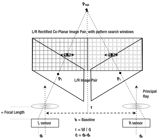
Binocular Stereo

Stereo [432, 433, 437] may be the most basic and familiar approach for capturing 3D depth maps, as many methods and algorithms are in use, so we provide a high-level overview here with selected standard references. The first step in stereo algorithms is to parameterize the projective transformation from world coordinate points to their corresponding image coordinates by determining the stereo calibration parameters of the camera system. Open-source software is available for stereo calibration.2_{Note that} the L/R image pair is rectified prior to searching for features for disparity computation. Stereo depth r is computed, as shown in Figure 1-10.

RGB TOF

1 2 3

4 5 6

7 8 9

L RGB RRGB

Ball Lens

Lens Array

Sensor Array

RGB

a. b.

c.

d.

e.

f.

Figure 1-9. A variety of lens and sensor configurations for common cameras:

a. conventional, b. time-of-flight, c. stereo, d. array, e. plenoptic, f. spherical with ball lens

(22)

Pxyz

b = Baseline

L/R Rectified Co-Planar Image Pair, with pattern search windows

L/R Image Pair

Pl Pr

L sensor R sensor

Principal Ray

f = Focal Length

r = bf / d d = dl-dr r

dl dr

Figure 1-10. Simplified schematic of basic binocular stereo principles

An excellent survey of stereo algorithms and methods is found in the work of Scharstein and Szeliski [440] and also Lazaros [441]. The stereo geometry is a combination of projective and Euclidean [437]; we discuss some of the geometric problems affecting their accuracy later in this section. The standard online resource for comparing stereo algorithms is provided by Middlebury College,3_{where many new} algorithms are benchmarked and comparative results provided, including the extensive ground truth datasets discussed in Appendix B.

(23)

The fundamental geometric calibration information needed for stereo depth includes the following basics.

• Camera Calibration Parameters. Camera calibration is outside the scope of this work, however the parameters are defined as 11 free parameters [435, 432]—3 for rotation, 3 for translation, and 5 intrinsic—plus one or more lens distortion parameters to reconstruct 3D points in world coordinates from the pixels in 2D camera space. The camera calibration may be performed using several methods, including a known calibration image pattern or one of many self-calibration methods [436]. Extrinsic parameters define the location of the camera in world coordinates, and

intrinsic parameters define the relationships between pixel coordinates in camera image coordinates. Key variables include the calibrated baseline distance between two cameras at the principal point or center point of the image under the optics; the focal length of the optics; their pixel size and aspect ratio, which is computed from the sensor size divided by pixel resolution in each axis; and the position and orientation of the cameras.

• Fundamental Matrix or Essential Matrix. These two matrices are related, defining the popular geometry of the stereo camera system for projective reconstruction [438, 436, 437]. Their derivation is beyond the scope of this work. Either matrix may be used, depending on the algorithms employed. The essential matrix uses only the extrinsic camera parameters and camera coordinates, and the fundamental matrix depends on both the extrinsic and intrinsic parameters, and reveals pixel relationships between the stereo image pairs on epipolar lines.

In either case, we end up with projective transformations to reconstruct the 3D points from the 2D camera points in the stereo image pair.

Stereo processing steps are typically as follows:

1. Capture: Photograph the left/right image pair simultaneously. 2. Rectification: Rectify left/right image pair onto the same plane,

so that pixel rows x coordinates and lines are aligned. Several projective warping methods may be used for rectification [437]. Rectification reduces the pattern match problem to a 1D search along the x-axis between images by aligning the images along the

x-axis. Rectification may also include radial distortion corrections for the optics as a separate step; however, many cameras include a built-in factory-calibrated radial distortion correction.

3. Feature Description: For each pixel in the image pairs, isolate a small region surrounding each pixel as a target feature descriptor.

(24)

4. Correspondence: Search for each target feature in the opposite image pair. The search operation is typically done twice, first searching for left-pair target features in the right image and then right-pair target features in the left image. Subpixel accuracy is required for correspondence to increase depth field accuracy.

5. Triangulation: Compute the disparity or distance between matched points using triangulation [439]. Sort all L/R target feature matches to find the best quality matches, using one of many methods [440].

6. Hole Filling: For pixels and associated target features with no corresponding good match, there is a hole in the depth map at that location. Holes may be caused by occlusion of the feature in either of the L/R image pairs, or simply by poor features to begin with. Holes are filled using local region nearest-neighbor pixel interpolation methods.

Stereo depth-range resolution is an exponential function of distance from the viewpoint: in general, the wider the baseline, the better the long-range depth resolution. A shorter baseline is better for close-range depth (see Figures 1-10 and 1-20). Human-eye baseline or inter-pupillary distance has been measured as between 50 and75mm, averaging about 70mm for males and 65mm for females.

Multi-view stereo (MVS) is a related method to compute depth from several views using different baselines of the same subject, such as from a single or monocular camera, or an array of cameras. Monocular, MVS, and array camera depth sensing are covered later in this section.

Structured and Coded Light

Structured or coded light uses specific patterns projected into the scene and imaged back, then measured to determine depth; see Figure 1-11. We define the following approaches for using structured light for this discussion [445]:

• Spatial single-pattern methods, requiring only a single illumination pattern in a single image.

(25)

For example, in the original Microsoft Kinect 3D depth camera, structured light consisting of several slightly different micro-grid patterns or pseudo-random points of infrared light are projected into the scene, then a single image is taken to capture the spots as they appear in the scene. Based on analysis of actual systems and patent applications, the original Kinect computes the depth using several methods, including (1) the size of the infrared spot—larger dots and low blurring mean the location is nearer, while smaller dots and more blurring mean the location is farther away; (2) the shape of the spot—a circle indicates a parallel surface, an ellipse indicates an oblique surface; and (3) by using small regions or a micro pattern of spots together so that the resolution is not very fine—however, noise sensitivity is good. Depth is computed from a single image

using this method, rather than requiring several sequential patterns and images. Multi-image methods are used for structured light, including projecting sets of time-sequential structured and coded patterns, as shown in Figure 1-11. In multi-image methods, each pattern is sent sequentially into the scene and imaged, then the combination of depth measurements from all the patterns is used to create the final depth map.

Industrial, scientific, and medical applications of depth measurements from structured light can reach high accuracy, imaging objects up to a few meters in size with precision that extends to micrometer range. Pattern projection methods are used, as well as laser-stripe pattern methods using multiple illumination beams to create wavelength interference; the interference is the measured to compute the distance. For example, common dental equipment uses small, hand-held laser range finders inserted into the mouth to create highly accurate depth images of tooth regions with missing pieces, and the images are then used to create new, practically perfectly fitting crowns or fillings using CAD/CAM micro-milling machines.

Of course, infrared light patterns do not work well outdoors in daylight; they become washed out by natural light. Also, the strength of the infrared emitters that can be used is limited by practicality and safety. The distance for effectively using structured light indoors is restricted by the amount of power that can be used for the IR emitters; perhaps a.

b.

c. d.

e.

f.

(26)

5 meters is a realistic limit for indoor infrared light. Kinect claims a range of about 4 meters for the current TOF (time of flight) method using uniform constant infrared illumination, while the first-generation Kinect sensor had similar depth range using structured light.

In addition to creating depth maps, structured or coded light is used for

measurements employing optical encoders, as in robotics and process control systems. The encoders measure radial or linear position. They provide IR illumination patterns and measure the response on a scale or reticle, which is useful for single-axis positioning devices like linear motors and rotary lead screws. For example, patterns such as the binary position code and the reflected binary gray code [444] can be converted easily into binary numbers (see Figure 1-11). The gray code set elements each have a Hamming distance of 1 between successive elements.

Structured light methods suffer problems when handling high-specular reflections and shadows; however, these problems can be mitigated by using an optical diffuser between the pattern projector and the scene using the diffuse structured light methods [443] designed to preserve illumination coding. In addition, multiple-pattern structured light methods cannot deal with fast-moving scenes; however, the single-pattern methods can deal well with frame motion, since only one frame is required.

Optical Coding: Diffraction Gratings

Diffraction gratings are one of many methods of optical coding [447] to create a set of patterns for depth-field imaging, where a light structuring element, such as a mirror, grating, light guide, or special lens, is placed close to the detector or the lens. The original Kinect system is reported to use a diffraction grating method to create the randomized infrared spot illumination pattern. Diffraction gratings [430,431] above the sensor, as shown in Figure 1-12, can provide angle-sensitive pixel sensing. In this case, the light is refracted into surrounding cells at various angles, as determined by the placement of the diffraction gratings or other beam-forming elements, such as light guides. This allows the same sensor data to be processed in different ways with respect to a given angle of view, yielding different images.

Photo-diodes

Gratings

(27)

This method allows the detector size to be reduced while providing higher resolution images using a combined series of low-resolution images captured in parallel from narrow aperture diffraction gratings. Diffraction gratings make it possible to produce a wide range of information from the same sensor data, including depth information, increased pixel resolution, perspective displacements, and focus on multiple focal planes after the image is taken. A diffraction grating is a type of illumination coding device.

As shown in Figure 1-13, the light-structuring or coding element may be placed in several configurations, including [447]:

Object side coding: close to the subjects •

Pupil plane coding: close to the lens on the object side •

Focal plane coding: close to the detector •

Illumination coding: close to the illuminator •

Detector

Detector Detector Detector

Optical Encoder + Illuminator Optical

Encoder Optical Encoder

Optical Encoder

Lens Lens

Figure 1-13. Various methods for optical structuring and coding of patterns [447]: (Left to right): Object side coding, pupil plane coding, focal plane coding, illumination coding or structured light. The illumination patterns are determined in the optical encoder

Note that illumination coding is shown as structured light patterns in Figure 1-11, while a variant of illumination coding is shown in Figure 1-7, using a set of mirrors that are opened or closed to create patterns.

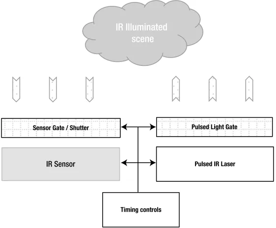
Time-of-Flight Sensors

By measuring the amount of time taken for infrared light to travel and reflect, a time-of-flight

(TOF) sensor is created [450]. A TOF sensor is a type of range finder or laser radar [449]. Several single-chip TOF sensor arrays and depth camera solutions are available, such as the second version of the Kinect depth camera. The basic concept involves broadcasting infrared light at a known time into the scene, such as by a pulsed IR laser, and then measuring the time taken for the light to return at each pixel. Sub-millimeter accuracy at ranges up to several hundred meters is reported for high-end systems [449], depending on the conditions under which the TOF sensor is used, the particular methods employed in the design, and the amount of power given to the IR laser.

(28)

capabilities. For example, by gating the electronic shutter to eliminate short round-trip responses, environmental conditions such as fog or smoke reflections can be reduced. In addition, specific depth ranges, such as long ranges, can be measured by opening and closing the shutter at desired time intervals.

IR Sensor

Sensor Gate / Shutter

Pulsed IR Laser Pulsed Light Gate

Timing controls

IR Illuminated scene

Figure 1-14. A hypothetical TOF sensor configuration. Note that the light pulse length and sensor can be gated together to target specific distance ranges

Illumination methods for TOF sensors may use very short IR laser pulses for a first image, acquire a second image with no laser pulse, and then take the difference between the images to eliminate ambient IR light contributions. By modulating the IR beam with an RF carrier signal using a photonic mixer device (PMD), the phase shift of the returning IR signal can be measured to increase accuracy—which is common among many laser range-finding methods [450]. Rapid optical gating combined with intensified CCD sensors can be used to increase accuracy to the sub-millimeter range in limited conditions, even at ranges above 100 meters. However, multiple IR reflections can contribute errors to the range image, since a single IR pulse is sent out over the entire scene and may reflect off of several surfaces before being imaged.

(29)

Array Cameras

As shown earlier in Figure 1-9, an array camera contains several cameras, typically arranged in a 2D array, such as a 3x3 array, providing several key options for computational imaging. Commercial array cameras for portable devices are beginning to appear. They may use the multi-view stereo method to compute disparity, utilizing a combination of sensors in the array, as discussed earlier. Some of the key advantages of an array camera include a wide baseline image set to compute a 3D depth map that can see through and around occlusions, higher-resolution images interpolated from the lower-resolution images of each sensor, all-in-focus images, and specific image refocusing at one or more locations. The maximum aperture of an array camera is equal to the widest baseline between the sensors.

Radial Cameras

A conical, or radial, mirror surrounding the lens and a 2D image sensor create a radial camera [413], which combines both 2D and 3D imaging. As shown in Figure 1-15, the radial mirror allows a 2D image to form in the center of the sensor and a radial toroidal image containing reflected 3D information forms around the sensor perimeter. By processing the toroidal information into a point cloud based on the geometry of the conical mirror, the depth is extracted and the 2D information in the center of the image can be overlaid as a texture map for full 3D reconstruction.

(30)

Plenoptics: Light Field Cameras

Plenoptic methods create a 3D space defined as a light field, created by multiple optics. Plenoptic systems use a set of micro-optics and main optics to image a 4D light field and extract images from the light field during post-processing [451, 452, 423]. Plenoptic cameras require only a single image sensor, as shown in Figure 1-16. The 4D light field contains information on each point in the space, and can be represented as a volume dataset, treating each point as a voxel, or 3D pixel with a 3D oriented surface, with color and opacity. Volume data can be processed to yield different views and perspective displacements, allowing focus at multiple focal planes after the image is taken. Slices of the volume can be taken to isolate perspectives and render 2D images. Rendering a light field can be done by using ray tracing and volume rendering methods [453, 454].

Subjects Main Lens Micro-Lens Array Sensor

Figure 1-16. A plenoptic camera illustration. Multiple independent subjects in the scene can be processed from the same sensor image. Depth of field and focus can be computed for each subject independently after the image is taken, yielding perspective and focal plane adjustments within the 3D light field

In addition to volume and surface renderings of the light field, a 2D slice from the 3D field or volume can be processed in the frequency domain by way of the Fourier Projection Slice Theorem [455], as illustrated in Figure 1-17. This is the basis for medical imaging methods in processing 3D MRI and CAT scan data. Applications of the Fourier Projection Slice method to volumetric and 3D range data are described by Levoy [455, 452] and Krig [137]. The basic algorithm is described as follows:

1. The volume data is forward transformed, using a 3D FFT into magnitude and phase data.

(31)

3. A planar 2D slice is extracted from the volume parallel to the FOV plane where the slice passes through the origin (center) of the volume. The angle of the slice taken from the frequency domain volume data determines the angle of the desired 2D view and the depth of field.

4. The 2D slice from the frequency domain is run through an inverse 2D FFT to yield a 2D spatial image corresponding to the chosen angle and depth of field.

Figure 1-17. Graphic representation of the algorithm for the Fourier Projection Slice Theorem, which is one method of light field processing. The 3D Fourier space is used to filter the data to create 2D views and renderings [455, 452, 137]. (Image used by permission, © Intel Press, from Building Intelligent Systems)

3D Depth Processing

For historical reasons, several terms with their acronyms are used in discussions of depth sensing and related methods, so we cover some overlapping topics in this section. Table 1-1 earlier provided a summary at a high level of the underlying physical means for depth sensing. Regardless of the depth-sensing method, there are many similarities and common problems. Post-processing the depth information is critical, considering the calibration accuracy of the camera system, the geometric model of the depth field, the measured accuracy of the depth data, any noise present in the depth data, and the intended application.

We survey several interrelated depth-sensing topics here, including:

Sparse depth-sensing methods •

Dense depth-sensing methods •

(32)

Simultaneous localization and mapping (SLAM) •

Structure from motion (SFM) •

3D surface reconstruction, 3D surface fusion •

Monocular depth sensing •

Stereo and multi-view stereo (MVS) •

Common problems in depth sensing •

Human depth perception relies on a set of innate and learned visual cues, which are outside the scope of this work and overlap into several fields, including optics, ophthalmology, and psychology [464]; however, we provide an overview of the above selected topics in the context of depth processing.

Overview of Methods

For this discussion of depth-processing methods, depth sensing falls into two major categories based on the methods shown in Table 1-1:

• Sparse depth methods, using computer vision methods to extract local interest points and features. Only selected points are assembled into a sparse depth map or point cloud. The features are tracked from frame to frame as the camera or scene moves, and the sparse point cloud is updated. Usually only a single camera is needed.

• Dense depth methods, computing depth at every pixel. This creates a dense depth map, using methods such as stereo, TOF, or MVS. It may involve one or more cameras.

Many sparse depth methods use standard monocular cameras and computer vision feature tracking, such as optical flow and SLAM (which are covered later in this section), and the feature descriptors are tracked from frame to frame to compute disparity and sparse depth. Dense depth methods are usually based more on a specific depth camera technology, such as stereo or structured light. There are exceptions, as covered next.

Problems in Depth Sensing and Processing

(33)

The Geometric Field and Distortions

Field geometry is a complex area affecting both depth sensing and 2D imaging. For commercial applications, geometric field problems may not be significant, since locating faces, tracking simple objects, and augmenting reality are not demanding in terms of 3D accuracy. However, military and industrial applications often require high precision and accuracy, so careful geometry treatment is in order. To understand the geometric field problems common to depth-sensing methods, let’s break down the major areas:

Projective geometry problems, dealing with perspective •

Polar and spherical geometry problems, dealing with perspective •

as the viewing frustum spreads with distance from the viewer

Radial distortion, due to lens aberrations •

Coordinate space problems, due to the Cartesian coordinates •

of the sensor and the voxels, and the polar coordinate nature of casting rays from the scene into the sensor

The goal of this discussion is to enumerate the problems in depth sensing, not to solve them, and to provide references where applicable. Since the topic of geometry is vast, we can only provide a few examples here of better methods for modeling the depth field. It is hoped that, by identifying the geometric problems involved in depth sensing, additional attention will be given to this important topic. The complete geometric model, including corrections, for any depth system is very complex. Usually, the topic of advanced geometry is ignored in popular commercial applications; however, we can be sure that advanced military applications such as particle beam weapons and missile systems do not ignore those complexities, given the precision required.

Several researchers have investigated more robust nonlinear methods of dealing with projective geometry problems [465,466] specifically by modeling epipolar geometry–related distortion as 3D cylindrical distortion, rather than as planar distortion, and by providing reasonable compute methods for correction. In addition, the work of Lovegrove and Davison [484] deals with the geometric field using a spherical mosaicking method to align whole images for depth fusion, increasing the accuracy due to the spherical modeling.

(34)

toward the boundaries of the depth field and less pronounced in the center. Some of the spherical distortion is due to lens aberrations toward the edges, and can be partially corrected as discussed earlier in this chapter regarding geometric corrections during early sensor processing.

Panum’s Area Horopter

Fused depth points

Figure 1-18. Problems with stereo and multi-view stereo methods, showing the Horopter region and Panum’s area, and three points in space that appear to be the same point from the left eye’s perspective but different from the right eye’s perspective. The three points surround the Horopter in Panum’s area and are fused by humans to synthesize apparent depth

Cartesian vs. Polar Coordinates: Spherical Projective

Geometry

(35)

Because stereo and MVS methods also use single 2D sensors, the same problems as affect single sensor depth-sensing methods also affect multi-camera methods, compounding the difficulties in developing a geometry model that is accurate and computationally reasonable.

Depth Granularity

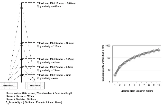
As shown in Figure 1-20, simple Cartesian depth computations cannot resolve the depth field into a linear uniform grain size; in fact, the depth field granularity increases exponentially with the distance from the sensor, while the ability to resolve depth at long ranges is much less accurate.

Sensor

P₁ P2

P3

(36)

For example, in a hypothetical stereo vision system with a baseline of 70mm using 480p video resolution, as shown in Figure 1-20, depth resolution at 10 meters drops off to about ½ meter; in other words, at 10 meters away, objects may not appear to move in Z unless they move at least plus or minus ½ meter in Z. The depth resolution can be doubled simply by doubling the sensor resolution. As distance increases, humans increasingly use monocular depth cues to determine depth, such as for size of objects, rate of an object’s motion, color intensity, and surface texture details.

Correspondence

Correspondence, or feature matching, is common to most depth-sensing methods. For a taxonomy of stereo feature matching algorithms, see Scharstein and Szeliski [440]. Here, we discuss correspondence along the lines of feature descriptor methods and triangulation as applied to stereo, multi-view stereo, and structured light.

Subpixel accuracy is a goal in most depth-sensing methods, so several algorithms exist [468]. It’s popular to correlate two patches or intensity templates by fitting the surfaces to find the highest match; however, Fourier methods are also used to correlate phase [467, 469], similar to the intensity correlation methods.

Y Pixel size: 480 / 10 meter = 20.8mm

Zy granularity = 465mm

Y Pixel size: 480 / 1 meter = 2mm

480p Sensor 480p Sensor

Stereo system, 480p sensors, 70mm baseline, 4.3mm focal length Sensor Y die size = .672mm

Sensor Y Pixel size: .0014mm

Zy Granularity = ( .0014mm * Z2_{mm) / ( 4.3mm * 70mm)}

Distance From Sensor in meters

Depth granularity or resolution in mmDep

th

granu

lar

ity

or reso

lu

tion

in m

m

(37)

For stereo systems, the image pairs are rectified prior to feature matching so that the features are expected to be found along the same line at about the same scale, as shown in Figure 1-11; descriptors with little or no rotational invariance are suitable [215, 120]. A feature descriptor such as a correlation template is fine, while a powerful method such as the SIFT feature description method [161] is overkill. The feature descriptor region may be a rectangle favoring disparity in the x-axis and expecting little variance in the y-axis, such as a rectangular 3x9 descriptor shape. The disparity is expected in the x-axis, not the

y-axis. Several window sizing methods for the descriptor shape are used, including fixed size and adaptive size [440].

Multi-view stereo systems are similar to stereo; however, the rectification stage may not be as accurate, since motion between frames can include scaling, translation, and rotation. Since scale and rotation may have significant correspondence problems between frames, other approaches to feature description have been applied to MVS, with better results. A few notable feature descriptor methods applied to multi-view and wide baseline stereo include the MSER [194] method (also discussed in Chapter 6), which uses a blob-like patch, and the SUSAN [164, 165] method (also discussed in Chapter 6), which defines the feature based on an object region or segmentation with a known centroid or nucleus around which the feature exists.

For structured light systems, the type of light pattern will determine the feature, and correlation of the phase is a popular method [469]. For example, structured light methods that rely on phase-shift patterns using phase correlation [467] template matching claim to be accurate to 1/100th_{of a pixel. Other methods are also used for structured light} correspondence to achieve subpixel accuracy [467].

Holes and Occlusion

When a pattern cannot be matched between frames, a hole exists in the depth map. Holes can also be caused by occlusion. In either case, the depth map must be repaired, and several methods exist for doing that. A hole map should be provided, showing where the problems are. A simple approach, then, is to fill the hole uses use bi-linear interpolation within local depth map patches. Another simple approach is to use the last known-good depth value in the depth map from the current scan line.

More robust methods for handling occlusion exist [472, 471] using more

computationally expensive but slightly more accurate methods, such as adaptive local windows to optimize the interpolation region. Yet another method of dealing with holes is surface fusion into a depth volume [473] (covered next), whereby multiple sequential depth maps are integrated into a depth volume as a cumulative surface, and then a depth map can be extracted from the depth volume.

Computer Vision Metrics