Christoph Böhm1, Odran Sourdeval2,3, Johannes Mülmenstädt2, Johannes Quaas2, and Susanne Crewell1
1Institute for Geophysics and Meteorology, University of Cologne, Cologne, Germany 2Institute of Meteorology, University of Leipzig, Leipzig, Germany
3Laboratoire d’Optique Atmosphérique, Université de Lille, Villeneuve-d’Ascq, France
Correspondence:Christoph Böhm ([email protected]) Received: 18 September 2018 – Discussion started: 5 October 2018
Revised: 21 February 2019 – Accepted: 22 February 2019 – Published: 20 March 2019
Abstract. Clouds are a key modulator of the Earth energy budget at the top of the atmosphere and at the surface. While the cloud top height is operationally retrieved with global coverage, only few methods have been proposed to determine cloud base height (zbase) from satellite measurements. This
study presents a new approach to retrieve cloud base heights using the Multi-angle Imaging SpectroRadiometer (MISR) on the Terra satellite. It can be applied if some cloud gaps oc-cur within the chosen distance of typically 10 km. The MISR cloud base height (MIBase) algorithm then determineszbase
from the ensemble of all MISR cloud top heights retrieved at a 1.1 km horizontal resolution in this area. MIBase is first cal-ibrated using 1 year of ceilometer data from more than 1500 sites within the continental United States of America. The 15th percentile of the cloud top height distribution within a circular area of 10 km radius provides the best agreement with the ground-based data. The thorough evaluation of the MIBase product zbase with further ceilometer data yields a
correlation coefficient of about 0.66, demonstrating the fea-sibility of this approach to retrievezbase. The impacts of the
cloud scene structure and macrophysical cloud properties are discussed. For a 3-year period, the median zbase is
gener-ated globally on a 0.25◦×0.25◦grid. Even though overcast cloud scenes and high clouds are excluded from the statis-tics, the medianzbaseretrievals yield plausible results, in
par-ticular over ocean as well as for seasonal differences. The potential of the full 16 years of MISR data is demonstrated for the southeast Pacific, revealing interannual variability in zbase in accordance with reanalysis data. The global cloud
base data for the 3-year period (2007–2009) are available at https://doi.org/10.5880/CRC1211DB.19.
1 Introduction
As Boucher et al. (2013) state in the IPCC Assessment Re-port 5, clouds and aerosols continue to contribute the largest uncertainty to estimates and interpretations of the Earth’s changing energy budget. To describe the effect of clouds on the radiation energy budget, the geometric thickness, the ver-tical location of clouds and, therefore, the cloud base height (zbase) are crucial parameters. Furthermore, long-term
obser-vations of cloud heights would be beneficial to assess the contribution and the response of clouds to climate change. zbaseis a key parameter for the radiative energy budget at the
Earth surface.zbase may also have an impact on ecosystems
which are supplied with water by the immersion of clouds (Van Beusekom et al., 2017). Aviation is another field which benefits from information onzbase.
Various methods to retrieve thezbasehave been proposed
applying different physical concepts, such as active measure-ments, spectral methods, approaches using an adiabatic cloud model (e.g., Goren et al., 2018) and in situ measurements.
From the ground, the most accurate and well-established method to derivezbaseis the backscatter information from a
lidar ceilometer, also providing crucial information on visi-bility for aircraft safety. Thus, ceilometers are employed at airports. Their number has increased in particular in Europe and North America during the past couple of years. A dedi-cated web page hosted by the Deutscher Wetterdienst shows the distribution of ceilometer stations around the world (http: //www.dwd.de/ceilomap, last access: 13 March 2019). Ra-diosondes provide in situ measurements of thermodynamic variables. Costa-Surós et al. (2014) compare different meth-ods to inferzbasefrom radiosonde data. For the best of these
uti-lized reference data regarding the number of cloud layers and height category (distinguished as low, middle and high). Cloud radar transmits microwave radiation to derive verti-cal profiles of radar reflectivity. However, this signal strongly depends on the particle size. Therefore, the occurrence of a few drizzle drops can mask the cloud base. Measurements with radiosondes and cloud radars are even less common than ceilometers; global coverage cannot be achieved from the ground today.
From space, active measurements are carried out by CALIOP (Cloud Aerosol Lidar with Orthogonal Polariza-tion) on the CALIPSO (Cloud Aerosol Lidar and Infrared Pathfinder Satellite Observations) satellite (Winker et al., 2010). A valid retrieval of the zbase can only be ensured if
the signal of CALIOP reaches the Earth’s surface, which is only possible in the case of low optical thickness. Optically thick clouds will lead to attenuation of the signal. The spa-tial coverage is limited to the narrow laser beam of CALIOP. The CALIOP cloud base determination has been revisited by Mülmenstädt et al. (2018). They developed an algorithm to extrapolate cloud base retrievals for thin clouds into locations where the CALIOP signal is attenuated within a thicker cloud before it reaches the cloud base.
Passive measurements in the near-infrared exploiting spec-tral information have been proposed by Ferlay et al. (2010). They suggest an approach to infer the cloud vertical extent from multi-angular POLDER (POLarization and Direction-ality of the Earth’s Reflectances) oxygen A-band measure-ments. As they point out, the penetration depth of photons into a cloud, and, hence, the height of the reflector, depends on the cloud vertical extent and the viewing geometry. Ex-ploiting the different viewing angles provided by POLDER, Desmons et al. (2013) apply this approach to infer the ver-tical position of clouds. Their comparison to retrievals from the cloud profiling radar on CloudSat and CALIOP shows that this method works best for liquid clouds over ocean with a retrieval bias of 5 m and a standard deviation of the retrieval differences of 964 m. However, this approach has not been carried out operationally yet. Moreover, an estimate of the cloud top height is required to retrieve the cloud base height from the cloud vertical extent, which introduces additional uncertainty.
Meerkötter and Zinner (2007) suggest a method to derive zbase of convective clouds which are not affected by
advec-tive motion. An adiabatic cloud model incorporating mea-surements of cloud optical depth and effective radius is used to calculate the geometric extent of the cloud from the re-trieved cloud top height. By introducing a subadiabatic fac-tor, Merk et al. (2016) investigate the adiabatic assumption in more detail. By additionally introducing a factor into the calculations, they account for subadiabaticity due to entrain-ment of dry air through the cloud edges. As a reference, the cloud vertical extent is derived as the difference betweenztop
(radar) and zbase (ceilometer) from ground-based
measure-ments. The authors conclude that for their 2-year data set,
neither the assumption of an adiabatic cloud nor the assump-tion of a temporally constant subadiabatic factor is fulfilled.
Lau et al. (2012) suggest a new approach to determine zbase utilizing the Multi-angle Imaging SpectroRadiometer
(MISR) on the Terra satellite. For a preliminary case study, they chose the observations from Graciosa Island, Azores, Portugal, for which they compared cloud top height (z) re-trievals from MISR to collocated and coincidental lidar mea-surements. Under the assumption that the cloud vertical ex-tent varies horizontally within the cloud, they retrievezbase
by identifying the lowest cloud top height in the height pro-file provided by MISR. The reference cloud base height (zˆbase) is retrieved from the lidar signal by visual inspection
of the backscatter coefficient in a time–height cross section over a period of about 5 h. They selected 12 cases which show a promising agreement between MISR and lidar re-trievals.
We build on the approach proposed by Lau et al. and develop an automatic retrieval method to derivezbase from
MISR measurements. Parameters employed in the retrieval scheme are derived from coincident ceilometer measure-ments over 1 year in the continental United States of Amer-ica (USA). The performance of thezbasealgorithm is
demon-strated through an evaluation with ceilometers over a longer time period, and the potential for application on the global scale and for longer time series is explored.
The paper is structured as follows. In Sect. 2, the utilized data from MISR and from ceilometers are described. Sec-tion 3 introduces the new retrieval method along with a case study for illustration. In Sect. 4, the evaluation of the algo-rithm against the ceilometer measurements is shown, and the effect of the scene structure on the performance of the algo-rithm is discussed. Section 5 includes two applications of the algorithm: the medianzbaseis presented globally for a 3-year
period and regionally over the southeast Pacific for a 16-year period. Finally, Sect. 6 concludes the study.
2 Data
2.1 MISR cloud product
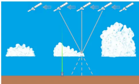
Figure 1.Schematic depiction of a cloud field observed from differ-ent viewing angles during the satellite overpass. Ceilometers, here represented as a cylindrical box, provide ground-based measure-ments of cloud base heights which can be used as a reference.
Here, we give a brief summary on how the operational MISR zproduct is derived. More in-depth descriptions can be found in Moroney et al. (2002) and in Marchand et al. (2007).
A cloud field is schematically depicted in Fig. 1. MISR hosts cameras providing a total of nine viewing angles. Be-sides the nadir viewing camera (0◦), there are four forward and four aftward-viewing cameras set up at 26.1, 45.6, 60.0 and 70.5◦ angles, respectively. During an overpass, each MISR camera records the reflected radiances at its particular viewing angle. A pattern matching routine which compares the radiances recorded at a wavelength of 670 nm identifies equal cloud features in the images of the different viewing angles. Pixels with the least deviation from each other are matched. This way, a detected cloud feature is observed from multiple satellite positions with its respective time and view-ing angle. If at least three images can be attributed to the same cloud feature, the cloud motion vector along with the horizontal and vertical position of the cloud feature can be inferred geometrically. This process is not sensitive to abso-lute values of the radiances; therefore, this retrieval method is not sensitive to calibration.
The cloud motion vector is determined at a 17.6 km reso-lution. For each of these coarser grid boxes, the cloud mo-tion vector is then used to determine z at 1.1 km resolu-tion, which is carried out for two camera pairs individually: one pair (FWD) consisting of the nadir and 26.1◦ forward-viewing cameras and the other (AFT) consisting of the nadir and 26.1◦aftward-viewing cameras. This way, twozvalues for the same location are available, and the mean of the two values yields the final z. In the case that only one camera pair provides a validz, it is taken as the finalzat its specific location. To derive the stereo-derived cloud mask, the two individual zvalues undergo the following comparison. The retrieval of each camera pair is classified as surface or cloud retrieval according to the threshold heighthmin(Eq. 1). This
is Eq. (59) in the Algorithm Theoretical Basis
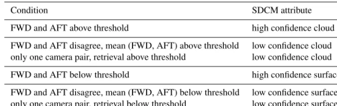
documenta-dence level to the retrievedz. If the mean of the two values is above or below the threshold, the pixel will be classified as cloud or surface, respectively. If only one camera pair pro-vides a valid retrieval, it is tested against the threshold and classified accordingly. In the case that only one camera pair provides a valid retrieval and in the case of two valid re-trievals which disagree upon their individual classification, thezretrieval is marked as having low confidence. If two re-trievals are available which agree upon their individual clas-sification, thezretrieval is marked as having high confidence. Any other case leads to a non-retrieval. Table 1 summarizes possible combinations of retrievals from the two camera pairs and their corresponding attribution within the stereo-derived cloud mask.
MISRzis given in meters above the World Geodetic Sys-tem 1984 (WGS 84) surface. To calculate the height above ground level, we subtract the average scene elevation, which is provided within the Ancillary Geographic Product for each pixel.
The MISRzproduct is expected to be superior toz prod-ucts from other passive instruments. It does not depend on any auxiliary data, and it is not sensitive to calibration. There-fore, it is not granted that the application of MIBase toz re-trieved using techniques other than the geometric approach would yield similar results.
2.2 METAR data
Aerodrome routine meteorological reports (METARs) (WMO; World Meteorological Organization, 2013) contain weather observations at airports worldwide, including mea-surements of zbase. METARs from airports from the
conti-nental USA providezbasedetermined by the Automated
near-Table 1.Classification scenarios of MISR retrievals. The cloud height obtained using the nadir and the 26.1◦forward-viewing camera pair (denoted by FWD) and the cloud height obtained using the nadir and the 26.1◦aftward-viewing camera pair (AFT) are tested against the threshold heighthmin(Eq. 1) individually and then compared to one another to determine the stereo-derived cloud mask (SDCM) attribute.
Condition SDCM attribute
FWD and AFT above threshold high confidence cloud
FWD and AFT disagree, mean (FWD, AFT) above threshold low confidence cloud only one camera pair, retrieval above threshold low confidence cloud
FWD and AFT below threshold high confidence surface
FWD and AFT disagree, mean (FWD, AFT) below threshold low confidence surface only one camera pair, retrieval below threshold low confidence surface
Table 2.The ceilometerzˆbaseretrievals are rounded to different val-ues depending on their height window according to ASOS User Guide (National Oceanic and Atmospheric Administration, De-partment of Defense, Federal Aviation Administration, and United States Navy, 1998). The values are originally given in feet and are converted to meters here.
Height (ft) Rounded to Rounded to
nearest value (ft) nearest value (m)
<5000 100 30.5
5000 to 10 000 500 152
>10 000 1000 305
est 500 ft (≈150 m) for heights above 10 000 ft (≈3000 m). If there are more than five bins filled with measurements dur-ing a 30 min period, the cloud heights are clustered into lay-ers until only five clustlay-ers remain. Finally, all cluster heights are rounded according to the rules given in Table 2. The low-est three layers are passed on to the METAR message.
We extract the ceilometer cloud base height zˆbase from
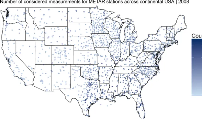
METAR data for a total of 1510 ceilometer sites around the continental USA to benefit from the homogeneity of the au-tomated measurements and the standardized reporting range.
ˆ
zbaseserves as reference data to which thezbasederived from
the satellite cloud heights is compared. First, METAR data from 2008 are used to estimate parameters used in thezbase
retrieval algorithm to create the MISR cloud base height algorithm (MIBase). Second, to validate the “tuned” algo-rithm, METAR data from 2007 are applied for a statisti-cally independent comparison. For a total of 1510 ceilometer stations, collocated and coincidental satellite-basedzbase
re-trievals could be found (see below for exact definition). A distribution of the locations can be seen in Fig. 2.
3 Cloud base height retrieval
The MISR cloud base height retrieval (MIBase) algorithm, which deriveszbase from the MISRzproduct, is developed
and calibrated with collocated METAR data to define the
pa-rameters and preconditions involved. The first subsection of this section introduces the retrieval principle on the basis of a case study. By comparison with METAR ceilometer mea-surements from 2008, parameters used within MIBase are estimated, namely the radiusRcof the MIBase retrieval cell,
the minimum number of valid cloud pixelN and the per-centileP of thezdistribution.
3.1 Method
We assume that the information on thezbaseis included in the
distribution of thezretrievals from the MISR cloud product for a specific area of limited size. This assumption is valid in a cloud scene with a homogeneouszbase and a
heteroge-neouszsimilar to the one schematically depicted in Fig. 1. Especially at the edge of a cloud where the cloud is thinner, zcan serve as a proxy forzbase. To ensure that the thinner
edge of the cloud is within the observed MIBase retrieval cell, the considered area needs to be large enough and the cloud field needs to be broken. The inherent assumption of a homogeneouszbase over a certain area presupposes a
hor-izontally constant lifting condensation level. This is a valid approximation in particular for a well-mixed boundary layer or a homogeneous air mass away from the proximity of a frontal zone, where advective motion could introduce tem-perature or humidity gradients across the horizontal plane.
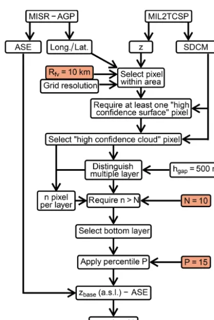
In order to derivezbase from thezproduct, the following
steps, which are outlined in Fig. 3, are undertaken. First, a retrieval cell has to be defined. For the comparison to the ceilometer measurements, we consider a circular area with the radiusRcaround its midpoint at a ceilometer station. In
order to estimate the magnitude ofRc, we consider the
fol-lowing: METARzˆbase retrievals are representative of a time
window of 30 min. Within this time window, and at a typical wind speed of approximately 10 ms−1, a cloud would shift its position about 20 km in the wind direction. Therefore, the magnitude ofRc should be on the order of kilometers. The
impact ofRc on the retrieved zbase and, therefore, the
de-viation from the ceilometerzˆbase is discussed below. When
Figure 2.Locations of ceilometer stations utilized in this study across the continental USA. Data from these stations for the years 2008 and 2007 are used for the calibration of thezbaseretrieval algorithm and a subsequent evaluation, respectively. Blue shading indicates the number of valid coincidental retrievals from MISR and ceilometers which were utilized for the calibration (year 2008) and are within the constraints described in the text.
we use a regular lat–long. grid of 0.25◦ (see Sect. 5). This grid size corresponds to a meridional length of the grid boxes of about 28 km and a zonal length ranging between 25 km (25◦N) and 18 km (50◦N), taking the continental USA as an example. A greater MIBase cell increases the chance of see-ing the thinner part of the cloud. This could lead to a more realisticzbaseretrieval. In turn, for a smaller MIBase cell, the
assumption of a homogeneouszbaseis more realistic.
For each grid cell or circular MIBase cell, the enclosedz retrievals from the MISR cloud product are processed further. MIBase only selects those zretrievals which are marked as high confidence cloud (hcc) according to the stereo-derived cloud mask. A consideration of retrievals marked as low con-fidence cloud (lcc) has shown a decrease of the correlation with the ceilometerzˆbase. An example of a cloud field with
zretrievals and the corresponding stereo-derived cloud mask for 21 August 2015 at the International Airport of Atlanta, Georgia, USA, is presented in Fig. 4a and b.
For some scenes, the distribution of z reveals extended height ranges with nozretrievals between two or more lo-cal maxima. Such cases suggest multilayer cloud scenes if the apparent gap between adjacentzretrievals is of sufficient size. If such a gaphgap is greater than 500 m, the algorithm
distinguishes between the cloud layer above and below the gap (see Fig. 4c for the aforementioned example). The value for this threshold has been chosen to be close to the specified accuracy of MISR (560 m). By evaluating different vertical cloud layers individually, azbaseretrieval for each layer can
be derived. Since for most applications the lowest zbase is
of interest, the lowest detected cloud layer is processed here.
For the comparison withzˆbase, we restrict ourselves to scenes
for which MISR detects only one cloud layer.
The occurrence of a broken cloud field is a basic require-ment of MIBase. Therefore, at least onezretrieval marked as high confidence surface needs to be within the MIBase cell. A complete cloud cover or a high rate of non-retrievals can prevent this criterion from being met. Both scenarios suggest doubtfulzbaseretrievals. Hence, they are not considered.
For each grid cell or circular cell surrounding the ceilome-ter station,zbaseis diagnosed from the height distribution of
zusing a certain percentileP. In principle,P should be as low as possible. However, as a certain measurement noise is expected and a robust result should be achieved, a choice substantially larger than zero is necessary. Another parame-ter which describes the distribution ofzfor each scene is the number of validzretrievals marked as high confidence cloud n. A highernimplies a higher observed cloud cover within the MIBase cell. In order to take a meaningful percentile of the zdistribution, a minimum n > N is required. A cloud which is horizontally more extended (higher cloud cover) is more likely to pass over the ceilometer. Therefore, there is a higher chance that both instruments observe the same cloud. Therefore, the deviation ofzbasefromzˆbaseis expected to
de-crease for a highern. The impact of the threshold forN is studied later on.
For certain applications, the cloud vertical extent1zmight be of interest. Therefore, an estimate of the cloud top height ztopis required. In principle,P =100 should yield the
high-est point of the cloud. However, analogously to the retrieval ofzbase, a certain measurement noise is expected. Therefore,
val-Figure 3. Flow chart of the zbase retrieval algorithm. MISR’s MIL2TCSP cloud product provideszand the stereo-derived cloud mask (SDCM). MISR’s Ancillary Geographic Product (MISR-AGP) provides the average scene elevation (ASE) and the longitude and latitude coordinates for each pixel. Starting from these prod-ucts, the processing steps depicted are undergone to derive zbase. The parameters which were optimized during the calibration are highlighted in orange.
idation, we apply the 95th percentile rather than the median, as we do not want a height which might be representative of the whole area but rather an estimate of the highest top of the cloud, especially for a heterogeneous cloud top height to estimate1zat its most extensive point.
3.2 Case study
One of the utilized ceilometer stations is located at the Hartsfield–Jackson Atlanta International Airport. To illus-trate the functionality of the presented algorithm, we investi-gate a particular MISR overpass over this station on 21 Au-gust 2015 at around 16:30 UTC. Figure 4 shows the z re-trievals for all pixels which are within the circular MIBase cell defined by Rc. Here, we exemplarily use Rc=20 km
with its midpoint at the ceilometer station.zis given above the WGS 84 surface, which is approximately equal to sea level. The spatial distribution shows a low cloud layer withz between 800 and 2000 m, which covers most of the area.
An-other cloud layer appears between 5 and 6 km. Some pixels with heights above 7 km indicate the presence of a third layer (Fig. 4a). For a few pixels, MISR was not able to determine z. This might be due to the viewing geometry. A retrieval requires valid images from two different cameras, one cam-era viewing nadir and the other viewing at a 26.1◦angle. In the case studied here, the most missing retrievals are closely attached to high clouds which might lead to shading effects (Fig. 4b).
The density of thezdistribution shows the aforementioned three cloud layers. They are distinguished according to the threshold value forhgap(Fig. 4c) as illustrated for the bottom
and middle layer. For the bottom layer, which is selected for further processing, the number ofzretrievals marked as high confidence cloud is determined to ben=621. This number is well above the thresholdN, which is defined later.zbaseis
then calculated usingP =15 as the preliminary percentile of thezdistribution. This yieldszbase≈1160 m above the WGS
84 surface. The mean average scene elevation for the given area is subtracted from the retrieval to obtainzbase≈927 m
above ground level. The closest METAR report for this day is from 16:52 UTC. Three heights were reported at 2800 ft (≈ 853 m), 7500 ft (≈2286 m) and 23 000 ft (≈7010 m) above ground level. By adding the station elevation (315 m), the corresponding height above sea level is obtained. This yields ˆ
zbase≈1168 m and is denoted in Fig 4c. In conclusion, using
the preliminary values forP, thezbase retrieval from MISR
is about 927 m above ground level, which is 74 m higher than the ceilometer retrieval (zˆbase=(853±15)m). The given
un-certainty solely represents the resolution of the METAR re-ports (Table 2). Note that the third layer detected around 7000 m by MISR was also detected by the ceilometer. 3.3 Parameter optimization
For each considered ceilometer station (Fig. 2), collocated and coincidental MISR overpasses from the year 2008 are identified. The algorithm is then applied as described in the case study (Sect. 3.2) to retrievezbase. All pairs of MIBase
zbaseand ceilometerzˆbaseare evaluated to investigate the
in-fluence ofRc,N andP on the performance of thezbase
re-trieval algorithm and to estimate the most suitable values. For this purpose, the following statistical measures are con-sidered: the slope and intercept of a linear regression, which are ideally 1 and 0, respectively; the Pearson correlation co-efficientr(ideally unity); the root mean square error (RMSE) E, defined as
E= v u u t
1 n
n X
i=1
zbase,i− ˆzbase,i 2
; (2)
and the retrieval biasB, defined as
B=1 n
n X
i=1
Figure 4.MISR observations within a 20 km radius within the vicinity of Atlanta, Georgia, USA (ICAO: KATL), on 21 August 2015 at around 16:30 UTC.(a)z.(b)Corresponding stereo-derived cloud mask (SDCM) distinguishing non-retrievals (NA), high confidence cloud (hcc), low confidence cloud (lcc), low confidence surface (lcs) and high confidence surface (hcs). (c)Density of zmeasurements with illustration of certain parameters: height between two layers (hgap), which is the height difference between the highest retrieval of the bottom layer and the lowest retrieval of the next higher layer (dashed blue lines); upper cutoff height (dashed orange) forzbaseretrievals (hmax), which is based on the ceilometer granularity; lower cutoff height (dashed red), which is based on the MISR threshold height to distinguish between cloud and surface retrieval (hmin); and the ceilometer retrievalzˆbasefrom 16:52 UTC (dashed pink).ztopandzbase(dashed purple) are inferred by applying the 15th and 95th percentile to the distribution ofzof the lowest cloud layer, respectively. Heights are above sea level.
Figure 5.Evaluation of the minimum number of valid pixelsNwithin a cloud layer detected by MISR for the year 2008.(a)The normalized number of events ns
nmax for whichzbaseandzˆbasecould both be retrieved.nmaxis the maximum number of events, which is found forN=1. (b)The linear correlation coefficientrbetweenzbaseandzˆbase.(c)The RMSE betweenzbaseandˆzbase. MISRzbaseis retrieved using the 15th percentile of thezdistribution for a 10 km radius around the individual ceilometer measurements. The chosen value forNis highlighted in orange. For further details, see text.
Table 3.Slope, intercept, correlation coefficientr, RMSEE, bias B and number of samplesns resulting from comparingzbaseand
ˆ
zbaseretrievals for different radii of the MISR circular area around the ceilometer stations. These values are obtained for the year 2008 applying a required minimum number of cloud pixels of N=10 and the 15th percentile to thezdistribution.
Rc Slope Intercept r E B ns
(km) (m) (m) (m)
5 0.65 371 0.66 392 −71 3059
10 0.62 412 0.66 404 −75 5120
15 0.60 433 0.65 413 −77 6140
20 0.58 464 0.63 423 −74 6895
30 0.54 515 0.60 437 −71 7772
MISR can only detect clouds above the threshold height according to Eq. (1). To prevent this obvious limitation from introducing a bias into the statistics, we only consider cloud scenes for which the ceilometer retrieval is above hmin. In
addition, onlyzbaseretrievals below a maximum heighthmax
of 3000 m are considered to focus on a cloud range for which the ceilometer retrievals are more finely granulated (below 10 000 ft according to Table 2).
First, we investigate the influence of the size of the MIBase cell on the comparison of MIBase and ceilometer retrievals. For this purpose,Rc is varied between 5 and 30 km, while
the other parameters are set to the preliminary valuesP =15 andN=10. With a decreasedRc, the correlation between
zbaseandzˆbaseincreases andEdecreases (Table 3). This is to
be expected as the representativity should increase. However, for a lowerRc, the retrieval algorithm encounters more
Figure 6.Evaluation of the percentileP which is applied to retrieve zbasefrom the distribution ofzfor the year 2008, withN=10 and Rc=10 km.(a)The linear correlation coefficientr betweenzbase andzˆbase.(b)The RMSE betweenzbaseandzˆbase. The chosen value forPis highlighted in orange.
high confidence surface pixel is visible and at least 10 valid cloud pixels per layer) cannot be fulfilled, as the decrease in the total number of retrievals indicates. The better agreement betweenzbase andzˆbasefor lowerRcmight be due to a
rel-atively larger overlap of the measurement sampling areas of the two instruments and to a better fulfilment of the assump-tion of a homogeneouszbaseover smaller areas. For further
evaluation, a radius of 10 km is chosen as a compromise be-tween a good agreement in terms of r andE and without having to discard too many retrieval scenes.
Second, the effect of the minimum number of validzbase
retrievals is studied, which strongly limits the number of samples for the comparison (Fig. 5). With increasingN, ini-tially a slight increase toN=10 improves the correlation be-tweenzbaseandzˆbaseandEsignificantly to a correlation
co-efficient of about 0.66. A further increase only yields slight improvement of the correlation andE. This slight increase can be explained by the elimination of more complex scenes from the comparison. However, for a higherN the trade-off is a lower total number ofzbase retrievals. For instance, for
N =50 only 80 % of possible retrievals yield a validzbase
(Fig. 5a). Therefore, we selectN=10.
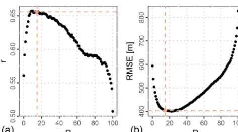
Finally, we consider the percentile threshold used to diag-nosezbasefrom thezdistribution. Figure 6 shows an
evalua-tion of different percentiles which are applied to derivezbase.
Percentiles between the 10th and the 15th give the best cor-relation. The lowest E is achieved for percentiles between the 15th and the 25th. Therefore,P =15 is chosen for fur-ther processing. The fact that very clear and localized minima (maxima) forE(r) are found supports the hypothesis that the zdistribution contains information onzbase.
In summary, the comparison yields the estimated parame-tersRc=10 km, the minimum numberN=10 and the
per-centileP =15. While the last two are kept fixed in MIBase, Rcis optimized for the intercomparison with point data, i.e.,
ceilometer measurements. The algorithm can also be applied
to larger grids. However, no data for validating extended ar-eas are available.
3.4 Scene limitations
This section investigates the applicability of MIBase by quantifying the number of cases for which the concurrent conditions allow the successful derivation of azbaseretrieval.
First, we filter for cases which fulfill the following two con-ditions: (i) the number of validzretrievals within the MIBase cellNvalmust be>0 and (ii) METAR data must be available
for the calibration and validation. These requirements are fulfilled for about two-thirds of all considered MISR over-passes over the ceilometer sites (Table 5). Furthermore, there are two main conditions which prevent the derivation of a zbase retrieval. These are namely apparent clear sky
condi-tions and apparent overcast, which is only a limitation for MIBase. Here, we use the phrases “apparent clear sky” and “apparent overcast” rather than “clear sky” and “overcast”, respectively, to account for the fact that this attribution is based on instrumental indications rather than actual known sky conditions.
For METAR, apparent clear sky is indicated if a METAR message is available but does not provide a valid retrieval. Note that in the case that the lowest cloud is above the METAR reporting range (typically 3700 m), it is possible that no retrieval is issued. Here, such cases would also be attributed apparent clear sky.
For MIBase, we attribute apparent clear sky to the fol-lowing configuration of the SDCM: MISR sees the surface with high confidence (NHCS>0) and has no high confidence
cloud in the view (NHCC=0). This does not have to be an
actual clear sky case since it could include low confidence surface or low confidence cloud retrievals, for which the dec-laration is less certain. In the case of invalidzretrievals, it is also uncertain whether clouds are present or not.
Out of all MISR apparent clear sky cases, 87 % are also classified as clear sky by METAR, while the remaining 13 % yield a METAR cloud height retrieval. Mismatches in at-tributing apparent clear sky cases are due to METAR re-trievals below the threshold heighthmin(17 %) and other
rea-sons, such as the temporal offset between MISR and METAR measurement. The METAR reports comprise retrievals over a 30 min period. During this time, cloud formation and cloud dissipation can alter the cloud scene and cause mismatches between MISR and METAR retrievals.
Furthermore, for MIBase, we attribute apparent overcast to the following configuration of the SDCM: MISR observes a cloud with high confidence (NHCC>0) and does not
ob-serve any surface retrievals with high confidence (NHCS=
Figure 7. (a, b)Joint density ofzbaseandzˆbasefor the year 2008(a, c)which is used to estimate parameters of the algorithm and for the year 2007(b, d)which is used to validate the stability of the algorithm with the estimated parameters. The value of the normalized density is indicated by color (maximum values in light yellow) and contour lines with corresponding values on them (linear scale). For each ceilometer height bin, the mean (red) and median (blue) of the MISRzbaseare shown.(c, d)Probability density functions of the residuals after a linear fit (red), the retrieval differences (blue) and a normal distribution with a standard deviation of 250 m (black).
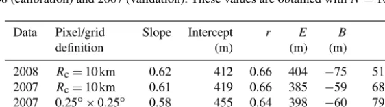
Table 4.Slope, intercept, correlation coefficientr, RMSEE, biasBand number of retrievalsnsresulting from a comparison ofzbaseand
ˆ
zbasefor data obtained in 2008 (calibration) and 2007 (validation). These values are obtained withN=10 andP=15.
Data Pixel/grid Slope Intercept r E B ns
definition (m) (m) (m)
2008 Rc=10 km 0.62 412 0.66 404 −75 5120
2007 Rc=10 km 0.61 419 0.66 385 −59 6801
2007 0.25◦×0.25◦ 0.58 455 0.64 398 −60 7970 2007 0.75◦×0.75◦ 0.49 579 0.55 446 −56 10 474
which the cloud cover is mainly above the reporting range of the ceilometer.
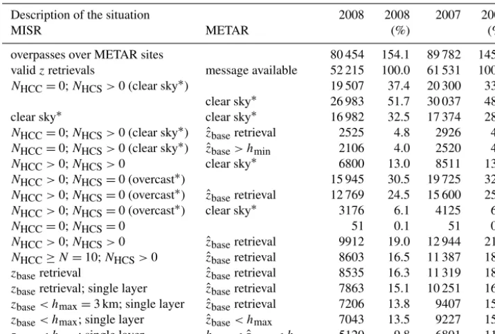
Out of all cases with validzretrievals within the MIBase cell (Nval>0) and a corresponding METAR retrieval, 19 %
are processed further. The main reasons why cases are ex-cluded are apparent clear sky scenes for MISR (37.4 %), ap-parent overcast for MISR (30.5 %) and apap-parent clear sky for METAR when valid zretrievals are within the MIBase
cell (13 %). Additional requirements, such as the minimum number of z retrievals marked as high confidence cloud (NHCC> N), single layer situations,zbaseandzˆbaseretrievals
belowhmaxand METAR retrievals above the MISR threshold
height (zˆbase> hmin), lead to a further reduction of the
Table 5.Number of cases for different conditions of the cloud field observed by MISR and reported in METAR messages for the considered METAR sites. The number ofzretrievals labeled “high confidence cloud” (NHCC) or “high confidence surface” (NHCS) according to MISR’s stereo-derived cloud mask is used to characterize the cloud field. The size of the scene is defined byRc=10 km.
Description of the situation 2008 2008 2007 2007
MISR METAR (%) (%)
overpasses over METAR sites 80 454 154.1 89 782 145.9
validzretrievals message available 52 215 100.0 61 531 100.0 NHCC=0;NHCS>0 (clear sky∗) 19 507 37.4 20 300 33.0
clear sky∗ 26 983 51.7 30 037 48.8
clear sky∗ clear sky∗ 16 982 32.5 17 374 28.2
NHCC=0;NHCS>0 (clear sky∗) zˆbaseretrieval 2525 4.8 2926 4.8 NHCC=0;NHCS>0 (clear sky∗) zˆbase> hmin 2106 4.0 2520 4.1
NHCC>0;NHCS>0 clear sky∗ 6800 13.0 8511 13.8
NHCC>0;NHCS=0 (overcast∗) 15 945 30.5 19 725 32.1 NHCC>0;NHCS=0 (overcast∗) zˆbaseretrieval 12 769 24.5 15 600 25.4 NHCC>0;NHCS=0 (overcast∗) clear sky∗ 3176 6.1 4125 6.7
NHCC=0;NHCS=0 51 0.1 51 0.1
NHCC>0;NHCS>0 zˆbaseretrieval 9912 19.0 12 944 21.0 NHCC≥N=10;NHCS>0 zˆbaseretrieval 8603 16.5 11 387 18.5
zbaseretrieval zˆbaseretrieval 8535 16.3 11 319 18.4
zbaseretrieval; single layer zˆbaseretrieval 7863 15.1 10 251 16.7 zbase< hmax=3 km; single layer zˆbaseretrieval 7206 13.8 9407 15.3 zbase< hmax; single layer zˆbase< hmax 7043 13.5 9227 15.0 zbase< hmax; single layer hmin<zˆbase< hmax 5120 9.8 6801 11.1 ∗indicates apparent conditions. See text for details.
4 MIBase evaluation
With the parameters Rc=10 km, N=10 and P =15
de-rived in the previous section, MIBase is applied to MISR re-trievals which are coincident with ceilometer rere-trievals from the year 2007. These data have not been used for calibra-tion. The joint density of zbase retrieved from MISR and
the ceilometer is shown in Fig. 7. For lower zbase, MISR
yields higher heights than the ceilometers. This can possi-bly be attributed to the threshold height (Eq. 1) constrain-ing zbase retrievals at the lower end of the height
distribu-tion. Forzbasegreater than 1000 m, mean and median MISR
heights are lower than the ceilometer. Overall, the biasB is slightly negative (about 60 m; cf. Table 4) and the density of the retrieval differences is shifted slightly towards negative values (Fig. 7d). Thus, MISR zbase retrievals are generally
lower than the ceilometer retrievals. This could be due to the different sample volumes. On the one hand, the ceilometer only records point measurements over a period of time, so the measured sample of the cloud depends on the velocity of the wind. On the other hand, MISR observes the entire circular area defined byRc around the ceilometer location. Chances
are that MISR can observe a cloud with a lower base which does not pass over the ceilometer.
The joint density and the density of the retrieval differ-ences appear similar for both the 2007 and the 2008 data sets (Fig. 7). Slope, intercept, r2,E, and B resulting from the zbase retrieval comparisons for the year 2008 (calibration)
and the year 2007 (validation) appear very similar, demon-strating the stability of the algorithm with the chosen pa-rameters (Table 4), to interannual variability in cloud proper-ties. Changing the MIBase cell to a 0.25◦×0.25◦ latitude– longitude grid results in a slightly lower correlation coef-ficient accompanied by a higher E. An even coarser grid size of 0.75◦×0.75◦, which is applied later for a compari-son with ERA-Interim cloud heights, results in an even lower correlation and higherE. A decreasing agreement between zbaseandzˆbasefor a larger MIBase cell has already been
de-scribed when studying the influence ofRc(see discussion in
Sect. 3.3).
4.1 Scene structure influence
To estimate the influence of the scene structure on the per-formance of MIBase, we further exploit the MISR cloud top height product and the MISR Ancillary Geographic Prod-uct to investigate characteristics of the terrain height and the cloud field.
To derive a quantity to estimate the variability of the ter-rain height, we calculate the standard deviation of the average scene elevation, which is provided by the ancillary product at 1.1 km resolution. For each METAR site, the standard devi-ation is calculated for an area defined by differentRc(5, 10,
Figure 8.From left to right: number of samplesns, RMSE, bias and correlation coefficientrfor the comparison of MIBase and ceilometer retrievals as a function of the number of validzretrievalsNval(panels a–d), the number of retrievals marked as high confidence surface NHCS(panels e–h) and the number of retrievals marked as high confidence cloudNHCC(panels i–l). Each data point is calculated for a subsample which includes onlyNval±δNval,NHCS±δNHCSandNHCC±δNHCC, respectively. The various widths of the consideredNval andNHCCwindows are indicated by the blue shading. All values are normalized by the total number of pixels within the MIBase cellNtot. Data are for the year 2008 withRc=10 km,P =15 andN=10.
sites with a higher standard deviation of the average scene elevation are excluded from the comparison of MIBase and METAR cloud base height retrievals, the RMSE decreases slightly and the bias slightly increases (towards 0), while the correlation is hardly affected (Fig. S1b, c, d). Thus, the vari-ability of the terrain height has a very small effect on the accuracy of the MIBase algorithm, with a slightly better per-formance over more homogeneous terrain.
To further investigate the performance of the MIBase al-gorithm as a function of parameters related to cloud types, we determine RMSE, bias and the correlation coefficient as a function ofztopand the cloud vertical extent1z(Fig. S2).
The best correlation is obtained for cloud vertical extents up to 1000 m. The RMSE is also smaller for lower1zand for lowerztop. However, the RMSE increases with
decreas-ingztopbelow about 1000 m. We conclude that MIBase
per-forms best for shallow low clouds. However, further analyses are necessary to increase the sample size of thicker clouds and to include more medium–high and high clouds for a more robust analysis of such cloud types. Furthermore, the increased RMSE for very lowztop indicates that, for very
Figure 9.Global distribution of median cloud heights for a 3-year period (2007–2009). Shown arezbase (a),ztop(b)and cloud vertical extent(d)on a 0.25◦×0.25◦latitude–longitude grid.zbaseandztopare above ground level (a.g.l.).zbaseandztopretrievals are only included in the statistic ifzbase is below 5000 m. The number of retrievalsns (c)represents the number of validzbaseretrievals within this 3-year period.
a shallow low cloud withzbaseandztopclose thehminwhen,
in fact, the actual cloud base is belowhmin. MIBase would
miss this actual cloud base height because the retrievals be-lowhminwould not be marked as high confidence cloud. For
that matter, we require that the ceilometer retrieval is above the threshold height (zˆbase> hmin). However, if such a
near-surface cloud was not detected by the ceilometer, a mismatch would result leading to a higher RMSE.
Additionally, we exploit the stereo-derived cloud mask as a proxy for the cloud cover fraction to investigate the sensi-tivity of the MIBase performance to the number of validz re-trievalsNval, the number ofzretrievals marked as high
confi-dence surfaceNHCSand the number ofzretrievals marked as
high confidence cloudNHCCwithin the MIBase cell. We
de-termine RMSE, bias and the correlation coefficient as a func-tion ofNval,NHCSandNHCCnormalized by the total number
of pixelsNtotwhich the MIBase cell encloses (Fig. 8). For
example, forRc=10 km, a total ofNtot=265 pixels is
pro-cessed by MIBase to obtain a uniquezbaseretrieval. For the
continental USA, most cases comprise a high portion of valid zretrievals within the MIBase cell. The RMSE, bias and the correlation coefficient are robust under different choices of Nval andNHCS. This suggests that MIBase generally does
not depend much on cloud cover fraction. However, for cases which suggest almost apparent clear sky, indicated by high NHCS, RMSE increases andr decreases. This could be due
to a lower chance of observing the same cloud in the case of less extended clouds. This bias appears to strongly
de-pend on the portion ofzretrievals marked as high confidence cloud (Fig. 8). The increased bias for higherNHCC could be
explained by the decreasing portion of the thin edge of the cloud compared to the thicker part of the cloud with greater horizontal extent. For instance, the edge of a larger cloud might only be partly within the MIBase cell, whereas the edge of a smaller cloud might be fully processed by MIBase. The clear increase of the bias with increasingNHCC shows
potential for a bias correction in the future after a better un-derstanding of the underlying reasons. The bias obtained in this study can have different sources: the different sample volumes of the defined MIBase cell and the ceilometer, bi-ased MISRzretrievals and various scene characteristics.
5 MIBase application
5.1 Global cloud height distribution
MIBase has been applied for a 3-year period between 2007 and 2009 to determine thezbasefrom MISR globally. Herein,
z data from each individual orbit have been sorted into a 0.25◦×0.25◦longitude by latitude grid. For each orbit and each grid box,zbase has been retrieved as described above
and the median over the 3-year period has been calculated. Only cloud height retrievals below 5000 m are considered to exclude cirrus clouds from the statistics.ztopis retrieved
Figure 10.Relative occurrences of different stereo-derived cloud mask (SDCM) configurations within the 3-year period (2007–2009). The reference sample sizensgiven in(a)corresponds to 100 % and includes all overpasses per grid cell which contain validzretrievals.(b) Rela-tive number for which MIBase successfully retrievedzbase. Panels(c)and(d)show the relative number of occurrence of cloud scenes which includezretrievals of specific SDCM labels within a grid cell. These configurations are(c)no high confidence cloud (HCS), which are apparent clear sky cases, and(d)no high confidence cloud (HCS), which are apparent overcast cases.
distribution. Taking the difference betweenztopandzbasefor
each observed cloud scene yields1z. The medians of these measures are shown in Fig. 9.
A sharp and steep gradient of thezbasecan be seen for most
coastlines with a higherzbase over land. This seems
plausi-ble as boundary layers above oceans are known to be shal-lower. Exceptions to this rule are the Congo Basin and the Amazon Basin. These regions are moisture sinks character-ized by high precipitation and excessive surface runoff. The maritime stratus cloud regions are clearly visible at the sub-tropical eastern boundaries of the Pacific, Atlantic and Indian oceans. These regions are characterized by prevailing high pressure due to the location at the subsiding branch of the Hadley circulation and cold ocean currents, creating a tem-perature inversion on top of the boundary layer. For these re-gions, cloud formation is limited to the well-mixed maritime boundary layer. The intertropical convergence zone (ITCZ) is clearly visible, in particular for the tropical Pacific Ocean with a higherzbase and even higherztop, yielding an overall
higher1zslightly north of the Equator. Over land, this phe-nomenon is not as clear. There, the diurnal cycle of surface heating becomes important. MISR on the Terra satellite has a morning overpass over the Equator when cloud formation just begins. Taylor et al. (2017) show the diurnal cycle of cloud top temperature (CTT) derived from SEVIRI measure-ments, indicating that the lowest ztop occurs between 9:00
and 13:00 local time with the lowest mean CTT at 11:00 and the lowest median CTT at 12:00, close to the overpass time of MISR.
The sampling size varies spatially, with a higher number of retrievals in the Arctic region. (Fig. 9c). This is expected for a polar orbiting satellite with more frequent MISR over-passes in polar regions (Fig. 10a). Generally, the causes for retrieval failure are apparent clear sky and apparent overcast situations, as discussed in Sect. 3.4. The frequency of occur-rence of such situations varies spatially. For continental dry regions in the subtropics and continental polar regions, ap-parent clear sky conditions predominantly limit the number of zbase retrievals (Fig. 10c). The continental polar regions
yield a high number of cases for which the grid cell com-prises only high confidence surface retrievals (NHCS=Ntot,
Fig. S3). This poses an even more robust indication of appar-ent clear sky conditions. However, the boundary layer is typ-ically shallower in polar regions. Therefore, boundary layer clouds occur likely belowhmin, sozbasecannot be retrieved
by the MIBase algorithm. Predominant apparent overcast conditions limit the number ofzbaseretrievals for midlatitude
regions over ocean and stratocumulus regions on the west-ern boundaries of continents in the subtropics. In midlatitude continental regions, a mix of apparent clear sky and apparent overcast conditions limits the number ofzbase retrievals. In
Figure 11.Global distribution of seasonal median cloud heights for a 3-year period (2007–2009). Shown areztop(a, b), andzbase(c, d)for December, January and February(a, c)and June, July and August(b, d)on a 0.25◦×0.25◦latitude–longitude grid.zbaseandztopare above ground level (a.g.l.).zbaseandztopretrievals are only included in the statistic ifzbaseis below 5000 m. The red rectangle in(d)frames the region for which results over a 16-year period are presented in Fig. 12.
success rates occur (Fig. 10b). A visual comparison to the 2011 mean cloud cover fraction derived from MODIS (Suen et al., 2014) indicates the plausibility of the attribution of ap-parent clear sky and apap-parent overcast.
To further investigate the plausibility of the seasonal vari-ability of cloud heights, composites over the 3-year period are presented in Fig. 11. We distinguish the boreal winter season comprising December, January and February (DJF) and the boreal summer season comprising June, July and August (JJA). Over land and between 30 and 70◦N,z
base
andztopare lower during winter, when stratiform clouds
pre-vail. In contrast, zbase and ztop are higher during summer,
when more convective clouds are typically present. Bound-ary layer clouds are also lower during the winter season since the boundary layer is shallower during the cold sea-son. Over ocean an inverse pattern can be observed in both hemispheres. During winter, zbase and ztop are higher than
during the summer. Sea surface temperatures show less sea-sonal variation than air temperatures due to the higher heat capacity of the water. This causes additional instability dur-ing winter, enhancdur-ing convective cloud formation, which can result in higher cloud heights. Additionally, the instability during winter can be attributed to storm tracks. During sum-mer, the influence of high-pressure systems can limit convec-tion to the maritime boundary layer, causing cloud heights to be lower.
5.2 Southeast Pacific
The southeast Pacific hosts one of the largest and most persis-tent stratocumulus cloud decks on Earth, as shown by Wood (2012) using data from the combined land–ocean cloud at-las database (Hahn and Warren, 2007). In this region, cloud cover and cloud thickness have major impacts on the net cloud radiative effect, which raises the importance of study-ing the heights of these clouds.
Orographically induced fog at the coastal cliff ranging from Peru to northern Chile is the major source of mois-ture for this region (Pinto et al., 2006). zbase and ztop of
the stratocumulus clouds near the coast determine the ar-eas where fog can provide water to the environment at the coastal cliff. The cloud heights also affect the ability of the fog to be advected further inland across the cliff. Here, we apply the zbase retrieval algorithm to determine the spatial
and seasonal variability ofzbaseandztopfor the region (see
red rectangle in Fig. 11d). We extend the time window to the full 16-year record of available MISR data (2001–2016). Furthermore, we investigate how well the temporal changes are represented in the global reanalysis ERA-Interim.
5.2.1 Spatial and seasonal variability ofzbaseandztop For the 16-year period, the medians of zbase andztop over
Figure 12.Median ofztop(a, b)andzbase(c, d)over a 16-year period (2001–2016) for austral summer (DJF,aandc) and austral winter (JJA,bandd) on a 0.25◦×0.25◦longitude by latitude grid in the southeast Pacific.zbaseandztopare given above ground level (a.g.l.). The red rectangle(d)frames the region for which a time series of cloud heights is presented in Fig. 13.
ranges from 600 m near the coast to about 1200 m further west. During austral summer (DJF) the lowest zbase is
ob-served near the coast between 30 and 35◦S. During austral winter the region of low zbase shifts to the north between
20 and 30◦S. This shift is in phase with the direction of the seasonal shift of the Hadley cell. It appears that the re-gion of lowestzbasecorresponds to the strongest subsidence.
During austral summer the highest zbase clearly appears in
the north, whereas during austral winter a north–south gra-dient is hardly visible between 120 and 80◦W. Over land, zbase is generally higher except for the coastline north of
35◦S, where cloud heights are even lower than over ocean. There, the prevailing maritime stratocumulus clouds form orographic fog as they reach the coastal cliff. Similar spatial and seasonal patterns are apparent for ztop. Over ocean, the
highestztopis about 2500 m, which is observed during
aus-tral summer in the northwest of the region. The lowestztopis
about 1000 m, which is observed during winter and closer to the coast of northern Chile.
5.2.2 Cloud height comparison between MISR and ERA-Interim
In order to preliminarily assess how well clouds are rep-resented in common reanalysis, we compare MISR-derived zbase and ztop to cloud heights derived from ERA-Interim
(Dee et al., 2011) which is provided by the European Cen-tre for Medium-Range Weather Forecasts (ECMWF). Cloud heights are not a direct output variable of ERA-Interim.
Therefore, the cloud liquid water content is used to infer the cloud base heightezbase and cloud top heighteztop. For
each grid point, the vertical column is scanned for model levels with a specific cloud liquid water content greater than 10−18kg kg−1(≈0). The bottom height of the lowest of such levels is taken asezbase. Moving higher in the column,eztopis
given by the bottom height of the next higher model level which has a cloud liquid water content equal to zero. We use data with a 0.75◦×0.75◦resolution, which is similar to the native grid of ERA-Interim, over a region between 20 and 23◦S and 74 and 71◦W, as indicated by the red rectangle in Fig. 12. ERA-Interim data are provided 6-hourly. The com-parison is performed using the 18:00 UTC output, which cor-responds to 14:00 Chile Standard Time (CLT). Note, MISR overpass times range around 10:51 to 11:29 CLT for this par-ticular region.
For each MISR overpass and ERA-Interim 18:00 UTC output, the median cloud heights are used to calculate the median cloud heights of each month over the whole 16-year period. The mean difference of the monthly cloud heights is roughly 500 m for both cloud base height and cloud top height, with ERA-Interim yielding lower cloud heights than MISR. The fact thatezbase is lower thanzbase could be due
to the threshold height used to determine the MISR stereo-derived cloud mask (Eq. 1), which leads to a cutoff ofzbase
retrievals athmin. At the same time the same bias is found
be-tweenztopandeztop. This could be an indicator that clouds are
mod-Figure 13.Time series of deviations of sea surface temperature1SST(a), cloud top height1ztop(b)and cloud base height1zbase(c)from the corresponding mean over the entire period from 2001 to 2016. Cloud heights are derived from MISR (green) and ERA-Interim (orange). SST is derived from ERA-Interim.
els typically underestimate the height of the planetary bound-ary layer (PBL) in the southeast Pacific area. This would cause boundary layer clouds to appear lower than observed. Their study compares the PBL height retrieved from in situ measurements and remote sensing to different models. While the observations show a PBL height of 1100 m, the models produce a PBL height between 400 and 800 m and hence an underestimation of 700 to 300 m. This is in accordance with the bias found here.
To reveal the annual cycle of the cloud heights, we look at anomalies from the 16-year mean of each time series (Fig. 13). These anomalies ofzbase andezbaseas well asztop
andeztopfrom their respective mean values agree rather well;
thus the amplitude of the annual cycle appears very similar. Figure 13 also shows the anomaly of the sea surface tempera-ture (SST) from its 16-year mean value. SSTs are taken from ERA-Interim as well. The peaks of the cloud heights corre-spond to the maxima of the SSTs. While the highest SSTs coincide with the highest cloud heights during austral sum-mer, the lowest SSTs coincide with the lowest cloud heights during austral winter.
6 Conclusions
Here, we present a new method to determinezbaseover a
spa-tial region from satellite-based measurements. The MIBase algorithm deriveszbasefrom the high spatial resolution MISR
cloud top height product zif some preconditions, such as a broken cloud scene, are met. Validation against 1510 ceilometer stations in the continental USA results in a cor-relation coefficient of 0.66 and a RMSE of 385 m for the val-idation data set (year 2007). The bias of−59 m even states
that MISR sees a slightly lowerzbaseon average. This is
pos-sibly due to the larger retrieval cell which is set up for the retrievals from MISR as opposed to the point measurements provided by the ceilometer.
Very few attempts to derivezbasefrom satellite have been
performed and evaluated before. Desmons et al. (2013) re-trieve 1zfrom POLDER measurements. The standard de-viation of the difference between their1zretrieval and ref-erence data from CPR and CALIOP is about 964 m. How-ever, their method is hard to compare to the MIBase al-gorithm, since they retrieve 1z and make a distinction of different types of clouds which is not done in this study. The CBASE algorithm (Mülmenstädt et al., 2018) derives zbase from CALIOP measurements, even for optically thick
clouds. Depending on the circumstances, different retrieval uncertainties can be derived. Similar to the study presented here, they compare theirzbaseretrievals with ceilometer data
over the continental USA. They obtain RMSEs between 404 and 720 m, depending on the concurrent local condi-tions of the individual retrievals. The RMSE we obtain for the MIBase algorithm is slightly lower. Even though the two studies make use of a similar reference database, they measure cloud heights at different times of the day. While CALIOP has an afternoon overpass, MISR has a morning overpass, when more clouds of lesser extent are present. For a more in-depth comparison and validation of the presented al-gorithm, more cloud height reference observations would be desirable, including observations in different climate zones and especially over ocean.
ity of the measurement, this newzbaseretrieval method is not
capable of deriving zbase below at least 560 m (flat terrain).
The algorithm requires a broken cloud scene. For complete overcast within the chosen MIBase cell,zbase cannot be
re-trieved. Therefore, climatologies derived from this algorithm would be biased towards cloud types for which MISR is able to observe the surface through cloud gaps.
Depending on the application, the MIBase uncertainty and the missing coverage of the diurnal cycle can be a limi-tation. However, in combination with ceilometer networks, both temporal and spatial patterns can be investigated. The application of MIBase over a 3-year period reveals plausi-ble patterns in the global distribution and seasonal variability of zbase. A first analysis over the 16-year MISR time series
in the southeast Pacific shows the potential to investigate the interannual variability ofzbase. This makes MIBase a
promis-ing tool for the evaluation of climate models on seasonal and interannual time scales in data-sparse regions if, for example, the climate model output is limited to clouds below 5 km and cloud fractions below 1 and if a sufficient number of MIBase retrievals is provided within the considered region and time period.
Appendix A: Sensitivity to threshold heighthmin
Figure A1.Joint density ofzbase andzˆbasefor the year 2008 ap-plying a lower threshold heighthmin=300 m+H+2σh(Eq. A1) for the distinction between surface and cloud pixels in contrast to Eq. (1).
The distinction between surface and cloud retrieval ac-cording to the threshold height described by Eq. (1) intro-duces a constraint to the zbase retrieval algorithm. Below a
height of 560 m for flat terrain, or higher for more complex terrain, zbase retrievals are not possible. As an attempt to
lower this threshold height, we adjusted HSDCM in Eq. (1)
so that
hmin=300 m+H+2σh. (A1)
acknowledge financial support by the Deutsche Forschungsge-meinschaft (DFG, German Research Foundation) – project number 268236062 – SFB 1211. We thank the seven referees for their constructive feedback.
Edited by: Alexander Kokhanovsky Reviewed by: seven anonymous referees
References
Böhm, C.: MIBase cloud base height derived from satellite data, data set, https://doi.org/10.5880/CRC1211DB.19, 2019. Boucher, O., Randall, D., Artaxo, P., Bretherton, C., Feingold, G.,
Forster, P., Kerminen, V.-M., Kondo, Y., Liao, H., Lohmann, U., Rasch, P., Satheesh, S., Sherwood, S., Stevens, B., and Zhang, X.: Clouds and Aerosols, in: Climate Change 2013: The Physi-cal Science Basis. Contribution of Working Group I to the Fifth Assessment Report of the Intergovernmental Panel on Climate Change, edited by: Stocker, T., Qin, D., Plattner, G.-K., Tig-nor, M., Allen, S., Boschung, J., Nauels, A., Xia, Y., Bex, V., and Midgley, P., chap. 7, 571–657, Cambridge University Press, Cambridge, United Kingdom and New York, NY, USA, 2013. Bull, M., Matthews, J., McDonald, D., Menzies, A., Moroney, C.,
Mueller, K., Paradise, S., and Smyth, M.: Data Products Spec-ifications, Tech. Rep. JPL D-13963, Revision S, Jet Propulsion Laboratory, California Institute of Technology, Pasadena, 2011. Costa-Surós, M., Calbó, J., González, J. A., and Long, C. N.:
Comparing the cloud vertical structure derived from several methods based on radiosonde profiles and ground-based re-mote sensing measurements, Atmos. Meas. Tech., 7, 2757–2773, https://doi.org/10.5194/amt-7-2757-2014, 2014.
Dee, D. P., Uppala, S. M., Simmons, A. J., Berrisford, P., Poli, P., Kobayashi, S., Andrae, U., Balmaseda, M. A., Balsamo, G., Bauer, P., Bechtold, P., Beljaars, A. C. M., van de Berg, L., Bid-lot, J., Bormann, N., Delsol, C., Dragani, R., Fuentes, M., Geer, A. J., Haimberger, L., Healy, S. B., Hersbach, H., Hólm, E. V., Isaksen, L., Kållberg, P., Köhler, M., Matricardi, M., McNally, A. P., Monge-Sanz, B. M., Morcrette, J.-J., Park, B.-K., Peubey, C., de Rosnay, P., Tavolato, C., Thépaut, J.-N., and Vitart, F.: The ERA-Interim reanalysis: configuration and performance of the data assimilation system, Q. J. Roy. Meteor. Soc., 137, 553–597, https://doi.org/10.1002/qj.828, 2011.
Desmons, M., Ferlay, N., Parol, F., Mcharek, L., and Van-bauce, C.: Improved information about the vertical location and extent of monolayer clouds from POLDER3 measurements in the oxygen A-band, Atmos. Meas. Tech., 6, 2221–2238, https://doi.org/10.5194/amt-6-2221-2013, 2013.
Goren, T., Rosenfeld, D., Sourdeval, O., and Quaas, J.: Satel-lite observations of precipitating marine stratocumulus show greater cloud fraction for decoupled clouds in comparison to coupled clouds, Geophys. Res. Lett., 45, 5126–5134, https://doi.org/10.1029/2018GL078122, 2018.
Haeffelin, M., Crewell, S., Illingworth, A. J., Pappalardo, G., Russchenberg, H., Chiriaco, M., Ebell, K., Hogan, R. J., and Madonna, F.: Parallel Developments and Formal Collab-oration between European Atmospheric Profiling Observato-ries and the U.S. ARM Research Program, Meteor. Mon., 57, 29.1–29.34, https://doi.org/10.1175/AMSMONOGRAPHS-D-15-0045.1, 2016.
Hahn, C. J. and Warren, S. G.: A gridded climatology of clouds over land (1971–96) and ocean (1954–97) from surface observations worldwide, Numeric Data Package NDP-026E ORNL/CDIAC-153, Tech. rep., CDIAC, Department of Energy, Oak Ridge, TN, https://doi.org/10.3334/CDIAC/cli.ndp026e, 2007.
Hannay, C., Williamson, D. L., Hack, J. J., Kiehl, J. T., Olson, J. G., Klein, S. A., Bretherton, C. S., and Köhler, M.: Eval-uation of Forecasted Southeast Pacific Stratocumulus in the NCAR, GFDL, and ECMWF Models, J. Climate, 22, 2871– 2889, https://doi.org/10.1175/2008JCLI2479.1, 2009.
Illingworth, A. J., Cimini, D., Haefele, A., Haeffelin, M., Hervo, M., Kotthaus, S., Löhnert, U., Martinet, P., Mattis, I., O’Connor, E. J., and Potthast, R.: How can Existing Ground-Based Profiling Instruments Improve European Weather Forecasts?, https://doi.org/10.1175/BAMS-D-17-0231.1, B. Am. Meteorol. Soc., in press, 2018.
Lau, M. W., Yung, Y. L., and Wu, D. L.: Determining Cloud Base and Thickness from Spaceborne Stereoscopic Imaging and Lidar Profiling Techniques, Caltech Undergraduate Research Journal, 12, 20–26, 2012.
Marchand, R. T., Ackerman, T. P., and Moroney, C.: An assessment of Multiangle Imaging Spectroradiometer (MISR) stereo-derived cloud top heights and cloud top winds using ground-based radar, lidar, and microwave radiometers, J. Geophys. Res.-Atmos., 112, D06204, https://doi.org/10.1029/2006JD007091, 2007. Meerkötter, R. and Zinner, T.: Satellite remote sensing of cloud base
height for convective cloud fields: A case study, Geophys. Res. Lett., 34, l17805, https://doi.org/10.1029/2007GL030347, 2007. Merk, D., Deneke, H., Pospichal, B., and Seifert, P.: Investigation of the adiabatic assumption for estimating cloud micro- and macro-physical properties from satellite and ground observations, At-mos. Chem. Phys., 16, 933–952, https://doi.org/10.5194/acp-16-933-2016, 2016.
Jet Propulsion Laboratory, California Institute of Technology, Pasadena, 2012.
Moroney, C., Davies, R., and Muller, J. P.: Operational retrieval of cloud-top heights using MISR data, IEEE T. Geosci. Remote, 40, 1532–1540, https://doi.org/10.1109/TGRS.2002.801150, 2002. Mueller, K., Moroney, C., Jovanovic, V., Garay, M., Muller,
J.-P., Di Girolamo, L., and Davies, R.: MISR Level 2 Cloud Product Algorithm Theoretical Basis, Tech. Rep. JPL D-73327, Jet Propulsion Laboratory, California Institute of Technology, Pasadena, 2013.
Mülmenstädt, J., Sourdeval, O., Henderson, D. S., L’Ecuyer, T. S., Unglaub, C., Jungandreas, L., Böhm, C., Russell, L. M., and Quaas, J.: Using CALIOP to estimate cloud-field base height and its uncertainty: the Cloud Base Altitude Spatial Extrapola-tor (CBASE) algorithm and dataset, Earth Syst. Sci. Data, 10, 2279–2293, https://doi.org/10.5194/essd-10-2279-2018, 2018. National Oceanic and Atmospheric Administration, Department of
Defense, Federal Aviation Administration, and United States Navy: Automated Surface Observing System User’s Guide, available at: https://www.weather.gov/media/asos/aum-toc.pdf (last access: 16 March 2019), 1998.
Pinto, R., Barría, I., and Marquet, P.: Geographi-cal distribution of Tillandsia lomas in the Atacama Desert, northern Chile, J. Arid Environ., 65, 543–552, https://doi.org/10.1016/j.jaridenv.2005.08.015, 2006.
Suen, J. Y., Fang, M. T., and Lubin, P. M.: Global Distri-bution of Water Vapor and Cloud Cover – Sites for High-Performance THz Applications, IEEE T. Thz. Sci. Techn., 4, 86– 100, https://doi.org/10.1109/TTHZ.2013.2294018, 2014. Taylor, S., Stier, P., White, B., Finkensieper, S., and
Sten-gel, M.: Evaluating the diurnal cycle in cloud top temper-ature from SEVIRI, Atmos. Chem. Phys., 17, 7035–7053, https://doi.org/10.5194/acp-17-7035-2017, 2017.
Van Beusekom, A. E., González, G., and Scholl, M. A.: Analyz-ing cloud base at local and regional scales to understand trop-ical montane cloud forest vulnerability to climate change, At-mos. Chem. Phys., 17, 7245–7259, https://doi.org/10.5194/acp-17-7245-2017, 2017.
Winker, D. M., Pelon, J., Coakley, J. A., Ackerman, S. A., Charlson, R. J., Colarco, P. R., Flamant, P., Fu, Q., Hoff, R. M., Kittaka, C., Kubar, T. L., Le Treut, H., Mccormick, M. P., Mégie, G., Poole, L., Powell, K., Trepte, C., Vaughan, M. A., and Wielicki, B. A.: The CALIPSO Mission, B. Am. Meteorol. Soc., 91, 1211–1230, https://doi.org/10.1175/2010BAMS3009.1, 2010.
Wood, R.: Stratocumulus Clouds, Mon. Weather Rev., 140, 2373– 2423, https://doi.org/10.1175/MWR-D-11-00121.1, 2012. World Meteorological Organization: Technical Regulations Volume