Computer Science Scholarship
Computer Science
2-2011
On-line planning and scheduling: an application to
controlling modular printers
Wheeler Ruml
University of New Hampshire, [email protected]
Minh Binh Do
Palo Alto Research Center
Rong Zhou
Palo Alto Research Center
Markus P. J. Fromherz
Palo Alto Research Center
Follow this and additional works at:
https://scholars.unh.edu/compsci_facpub
Part of the
Computer Sciences Commons
This Article is brought to you for free and open access by the Computer Science at University of New Hampshire Scholars' Repository. It has been accepted for inclusion in Computer Science Scholarship by an authorized administrator of University of New Hampshire Scholars' Repository. For more information, please [email protected].
Recommended Citation
On-line Planning and Scheduling:
An Application to Controlling Modular Printers
Wheeler Ruml ruml at cs.unh.edu
Department of Computer Science University of New Hampshire 33 Academic Way
Durham, NH 03824 USA
Minh Binh Do minhdo at parc.com
Rong Zhou rzhou at parc.com
Markus P. J. Fromherz fromherz at parc.com
Palo Alto Research Center 3333 Coyote Hill Road Palo Alto, CA 94304 USA
Abstract
We present a case study of artificial intelligence techniques applied to the control of production printing equipment. Like many other real-world applications, this complex do-main requires high-speed autonomous decision-making and robust continual operation. To our knowledge, this work represents the first successful industrial application of embedded domain-independent temporal planning. Our system handles execution failures and multi-objective preferences. At its heart is an on-line algorithm that combines techniques from state-space planning and partial-order scheduling. We suggest that this general architec-ture may prove useful in other applications as more intelligent systems operate in continual, on-line settings. Our system has been used to drive several commercial prototypes and has enabled a new product architecture for our industrial partner. When compared with state-of-the-art off-line planners, our system is hundreds of times faster and often finds better plans. Our experience demonstrates that domain-independent AI planning based on heuristic search can flexibly handle time, resources, replanning, and multiple objectives in a high-speed practical application without requiring hand-coded control knowledge.
1. Introduction
the same equipment. A printer controller must plan quickly and reliably; otherwise expen-sive human intervention will be required. Designing a high-performance yet cost-effective controller for such machines is made more difficult by the current trend towards increased modularity, in which each customer’s system is unique and includes only those components that are most appropriate for their needs. We have been working closely with the Xerox Corporation to explore architectures in which printing systems can be composed of liter-ally hundreds of modules, possibly including multiple specialized printing modules, working together at high speed.
In this paper, we demonstrate how techniques from artificial intelligence can be used to control such machines. Requests for print jobs become goals for the system to achieve, the various actuators and mechanisms in the machine become actions and resources to be used in achieving these goals, and sensors provide feedback on action execution and the state of the system. To provide high productivity (and thus high return on investment for the equipment owner), the planning and control techniques must be fast and produce optimal or near-optimal plans. To reduce the need for operator oversight and to allow the use of very complex mechanisms, the system must be as autonomous and autonomic as possible. Because operators can make mistakes and even highly-engineered system modules can fail, the system must cope with execution failure and unexpected events. And because the system must work with legacy modules in order to be commercially viable, its architecture must tolerate components that are out of its direct control.
To meet these requirements, we present a novel architecture for on-line planning, execu-tion, and replanning that synthesizes techniques from state-space planning (Ghallab, Nau, & Traverso, 2004) and partial-order scheduling (Smith & Cheng, 1993). We develop new heuristic evaluation functions for temporal planning that incorporate some of the effects of resource constraints. Although domain-independent AI planning is often regarded as too expensive for use in a soft real-time setting, our system achieves good performance without any hand-coded control rules, despite the additional requirements of reasoning about tem-poral actions and resources. By avoiding domain-dependent search control knowledge, it becomes possible to use the same planner to run very different printing systems at full pro-ductivity. The success of our system has enabled a new modular product architecture that can span multiple markets. Much as previous work brought constraint-based scheduling into daily use in print shops and offices world-wide (Fromherz, Saraswat, & Bobrow, 1999; Fromherz, Bobrow, & de Kleer, 2003), our work can bring domain-independent temporal planning into continual widespread use by everyday people. Our approach is practical and efficient, and it showcases the flexibility inherent in viewing planning as heuristic search.
Figure 1: A prototype modular printer built at PARC. The system is composed of approx-imately 170 individually controlled modules, including four print engines.
We conclude the paper with a summary of general lessons we derived from building this application.
2. Application Context
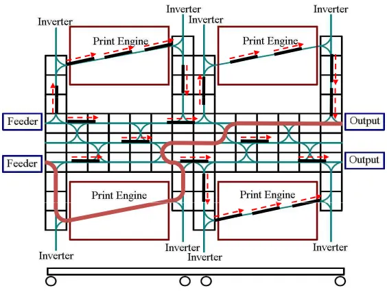
Figure 2: A schematic side view of the modular printer indicating the feeders, paper path, and output trays.
components to add new modules and functionality. Achieving these benefits, however, poses a considerable control challenge.
The modular printing domain is reminiscent of ‘mass customization,’ in which mass-produced products are closely tailored and personalized to individual customers’ needs. It is also similar to package routing or logistics problems. From a control perspective, it involves planning and scheduling a series of sheet requests that arrive asynchronously over time from the front-end print-job submission and rendering engine. The system runs at high speed, with several sheet requests arriving per second, possibly for many hours. Each sheet request completely describes the attributes of a desired final product. There may be several different sequences of actions that can be used to print a given sheet. For example, in Figure 2, a blank sheet may be fed from either of the two feeders, then routed to any one of the four print engines (or through any combination of two of the four engines in the case of duplex printing) and then to either finisher (unless the sheet is part of an on-going print job).
T ra n sl at o r sheet description printer model Planner STN Plan Manager domain description problem description goals plans constraints failures time info Machine Controller itineraries rejections, failures, updates T ra n sl at o r
Figure 3: The system architecture, with the planning system indicated by the dashed box.
The planning system must decide how to print all requested sheets as quickly as possible and thus it must determine a plan and schedule for each sheet such that the end time T of the plan that finishes last is minimized. In other words, the planner attempts to minimize the makespan of the combined global plan for all sheets, in essence optimizing the system’s overall throughput. Typically there are many feasible plans for any given sheet request; the problem is to quickly find one that minimizesT. The optimal plan for a sheet depends not only on the sheet request, but also on the resource commitments present in previously-planned sheets. Any legal series of actions can always be easily scheduled by pushing it far into the future, when the entire printer has become completely idle, but of course this is not desirable. This is an on-line task because the set of sheets grows as time passes and plan execution (i.e., printing) interleaves with plan creation. In fact, because it is the real-world wall clock end time that we want to minimize and because the production of a sheet cannot start until it is planned, the speed of the planner itself affects the value of a plan! However, the system often runs at full capacity, and thus the planner usually need only plan at the rate at which sheets are completed, which again may be several per second. While challenging, the domain is also forgiving: feasible schedules can be found quickly, sub-optimal plans are acceptable, and plan execution is relatively reliable.
sheet 1 sheet 2 sheet 4
sheet 5
sheet
d
i ti
st
ar
t t
i
sheet 3 sheet 4
sheet 5 sheet 6
sheet 7
descriptions
m
e
sent to
printer
planned,
unsent
being
planned
not yet
planned
Figure 4: Stages in the life of a sheet in the planning system.
close enough to the current wall-clock time and send those plans to the printer controller for execution (sheets 1 and 2). Note that in the figure, time advances downward so plans starting earlier are higher in the figure. Sheets 1, 2, and 3 finish in order; sheets 4 and 5 belongs to a different job and can be scheduled to run concurrently.
In our application, there is an additional negotiation step after a plan is issued by the planning system and before the plan is committed. First, each plan step isproposed by the machine controller to the modules involved. If the individual hardware modules from all stepsaccept their proposed actions, then the plan is committed. As we discuss below, this commitment means that modules become responsible for notifying the controller if they fail to complete an action or realize that they will not be able to perform a planned action in the future. After a plan is confirmed, the planner cannot modify it. There is thus some benefit in releasing plans to the machine controller only when their start times approach. If not all modules confirm, then the machine controller notifies the planning system that the proposed plan has been rejected, and the system must produce a new plan. This negotiation process is one reason that we must find a complete plan before starting execution.
Each module has a limited number of discrete actions it can perform, each transforming a sheet in a known deterministic way. For many of these actions, the planner is allowed to control its duration within a range spanning three orders of magnitude (milliseconds to seconds). For example, the planner may choose to transport a sheet faster or slower through a module in order to avoid collisions. Actions may not split a sheet into two pieces or join multiple sheets from different paths in the printer together. This means that a single printed sheet must be created from a single blank sheet of the same size, thereby conflating sheets with material and allowing plans to be a linear sequence of actions. In our domain, adjacent actions must meet in time; sheets cannot be left lingering inside a printer after an action has completed but must immediately begin being transported to its next location.
jobs are not allowed to interleave at a single destination, the number of concurrent jobs is limited by the number of destinations (i.e., finisher trays).
Currently, Xerox uses a constraint-based scheduler to control its high-end and mid-range printers (Fromherz et al., 1999). The scheduler enumerates all possible plans when the machine starts up and stores them in a database. When printing requests arrive on-line, the scheduler picks the first feasible plan from the database and uses temporal constraint processing to schedule its actions. This decoupling of planning and scheduling is insufficient for complex machines for two reasons. First, the number of possible plans is too large to generate ahead of time, and indeed becomes infinite if loops are present, as in the printer shown in Figure 2. Second, the precompiled plans can be poor choices given the existing sheets in the system. For example, sheets should be fed from different feeders depending on when the previous sheets were fed, how large they are, and how long they will dwell in the print engines (which can be a function of sheet thickness and material). For high performance, we must integrate planning and scheduling in an on-line fashion.
Occasionally a module will break down, failing to perform its committed action. Modules can also take themselves off-line intentionally, for example to perform internal re-calibration or diagnosis. Modules may be added or subtracted from the system and this information is passed from the machine controller to the planning system at the right side of Figure 3. The vision of RMP is that the system should provide the highest possible level of productivity that is safe, including running for long periods with degraded capabilities.1 Meeting this mandate in the context of highly modular systems means that precomputing a limited set of canonical plans and limiting on-line computation to scheduling only is not desirable. For a large system of 200 modules, there are infeasibly many possible degraded configurations to consider. Depending on the capabilities of the machines, the number of possible sheet requests may also make plan precomputation infeasible. Furthermore, even the best pre-computed plan for a given sheet may be suboptimal given the current resource commitments in the printing machine.
To summarize, our domain is finite-state, fully-observable, and specifies classical goals of achievement. However, planning is on-line with additional goals arriving asynchronously. Actions have real-valued durations and use resources. Plans for new goals must respect resource allocations of previous plans. Execution failures and domain model changes can occur on-line, but are rare.
3. System Overview
A complete printing system encompasses many components, including print-job submission, print-job management and planning, sheet management and planning, image rendering and distribution, low-level module control, media handling hardware, and exception handling. This paper focuses on planning issues at the sheet level, including exception handling. Before discussing any one issue in great detail, this section provides an overview of those topics that involve sheet planning most directly, including hardware control and exception handling.
Feed
Loop
Finish
1 2
1 2
1 2
2
2
2 1
2 1
2 2
1 2
1 2 3 4 5 6 1 2 3 4 5
Time Step
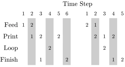
Figure 5: Two different schedules for printing a duplex sheet (2) after a simplex sheet (1): launching the sheets out of order improves throughput.
Figure 3 shows the basic architecture of the planning system and how it communicates with the machine controller. The overall objective is to minimize the makespan of the combined global plan for all sheets, in essence optimizing the system’s throughput. We approximate this by planning one sheet at a time, with the objective of having that sheet finish as quickly as possible while respecting any ordering constraints it may have with other sheets. Sheets are optimally planned on an individual basis, in order of arrival, without reconsidering the plans selected for previous sheets. In the figure, the plan manager calls the planner for each sheet and records the resulting plan. To mitigate the restrictiveness of this greedy scheme, we represent action times using temporal constraints instead of absolute times. These constraints are stored in a simple temporal network (Dechter, Meiri, & Pearl, 1991), marked STN in the figure. By maintaining temporal flexibility as long as possible, we can shift plans for older sheets later in time to make room for starting a new sheet earlier if that improves overall machine throughput. While this may sound like a rare case, it can be quite common. Figure 5 illustrates how, for a simplex (single-sided) cover sheet followed by a duplex (double-sided) sheet, it can be faster overall to launch the second sheet first.
Although this basic architecture is specifically adapted to our on-line setting, the plan-ner uses no domain-dependent search control knowledge. Furthermore, this mix of goal-decomposable planning with cross-goal resource constraints is quite common, and we believe our framework can be useful in any AI system that needs to interleave real-time decision making, planning, and execution, such as robot operations.
3.1 Planning
On-linePlanner
1. plan the next sheet
2. if an unsent plan starts soon, then
3. foreach plan, from the oldest through the imminent one 4. clamp its time points to the earliest possible times 5. release the plan to the machine controller
PlanSheet
6. search queue← {final state}
7. loop:
8. dequeue the most promising node 9. if it is the initial state, then return 10. foreach applicable action
11. apply the action
12. add temporal constraints
13. foreach potential resource conflict
14. generate all orderings of the conflicting actions 15 enqueue any feasible child nodes
Figure 6: Outline of the hybrid planner
the backward state-space search, it can be seen as a hybrid between state-space search and partial-order planning. A sketch of the planner is given in Figure 6. The outer loop corresponds to the plan manager in Figure 3.
After planning a new sheet, the outer loop checks the queue of planned sheets to see if any of them begin soon (step 2). It is imperative to recheck this queue on a periodic basis, so ‘soon’ is defined to be before some constant amount after the current time and we assume that the time to plan the next sheet will be smaller than this constant. The value of this constant depends on the domain specifics such as communication delay or module preparation time and is currently selected manually. If this assumption is violated, we can interrupt planning the next sheet and start over later. As plans are released and executed, resource contention will only decrease, so the time to plan the new sheet should decrease as well. It is important that new temporal constraints are added by the outer loop only between the planning of individual sheets, as propagation can affect feasible sheet end times and thus could invalidate previously computed search node evaluations if planning were underway.
to be due mainly to the temporal constraint enforcing that a given sheet should end after the end time of all the previous sheets in the same batch. This constraint interacts well with searching backward from the goal, immediately constraining the end time of the plan. Together with the constraint that actions must abut in time, many possible orderings for resolving resource contention are immediately ruled out. For example, the current sheet cannot be transported to its destination before the previous sheet in the same batch. In addition, some orderings may immediately push the end time of the plan even later, further informing the node evaluation function.
A planner that searches in the forward direction benefits slightly from avoiding logical states that are unreachable from the initial state. However, without a similar temporal constraint for the first action in the plan, few resource allocation orderings can be pruned and the branching due to resource contention increases in direct proportion to the number of plans for previous sheets maintained in the plan manager. Furthermore, the end time of the plan rarely changes until far into the planning processes, making the heuristic less useful. In short, for the first sheet, the performance of forward or backward planners are similar, while as the number of plans managed by the plan manager increases, the backward planner seems to perform better.
Due to details of the machine controller software, the planner must release plans to the machine controller in the same order in which the sheet requests were submitted. This means that sheets submitted before any imminent sheet must be released along with it (step 3). Only at this stage are the allowable intervals of the sheet’s time points forcibly reduced to specific absolute times (step 4). Sensibly enough, we ask that each point occur exactly at the earliest possible time. Because the temporal network uses a complete algorithm to maintain the allowable window for each time point (a variation on Cervoni, Cesta, & Oddi, 1994), we are guaranteed that the propagation caused by this temporal clamping process will not introduce any inconsistencies. The clamping happens before plans are issued; thus we do not face the on-line dispatchability problem of Muscettola, Morris, and Tsamardinos (1998).
In our current on-line setting, even though we plan for multiple sheets belonging to different jobs, we build plans for a single sheet at the time. Even if there are many submitted sheets waiting to be planned, this strategy is reasonable given that sheets arrived in sequence and, until the arrival of the last sheet, we do not know how many sheets are in each job and when the planner will receive the individual sheet specifications. Waiting until all sheets are known is impractical as many production jobs, such as billing and payroll, involve jobs with many thousands of sheets that can run for multiple days.
3.2 Control
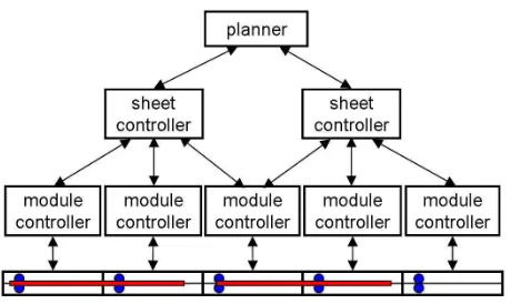
Figure 7: The control system architecture.
DSP. All modules run the same distributed algorithms for state estimation and control and communicate with each other via five controller-area network (CAN) buses, plus a dedicated data-logging bus for debugging purposes. Modules from the same ‘quadrant’ of the printer reside on the same CAN bus, except for the four print engines, which are on a separate bus. Sheets are moved by roller actuators, called nips, that are driven by independently-controlled stepper motors. For sensory feedback, each nip is equipped with an edge-detection sensor on both sides of the nip. In each three-way module, there are three solenoids that drive flipper actuators to direct the sheet along different paths.
Figure 7 shows the control system architecture, which implements a hierarchical ap-proach to distributed plan execution in which a sheet controller manages those module controllers that are currently, or will soon be, in contact with the sheet. Thus the sheet controller group membership is dynamic over the life cycle of a sheet, starting from the feeder all the way to the finisher tray. As soon as a new sheet is sent to the machine con-troller, a corresponding sheet controller is created that resides on a centralized processor, even though all the module controllers it manages reside locally on the modules themselves. Note that a module controller may be processing commands from multiple sheet controllers, as is the case of the module controller in the middle of Figure 7. While still in contact with the first sheet, it will soon be in contact with the second sheet.
for communications (Crawford, Hindi, Zhou, & Larner, 2009; Hindi, Crawford, & Fromherz, 2005).
The limited network bandwidth has fundamental impact on our choice of the control al-gorithm. Initially, a linear-quadratic-gaussian (LQG) (Franklin, Powell, & Workman, 1997) controller was used, which has the nice property that its solution constitutes a linear dy-namic feedback control law that is easily computed. However, the bandwidth requirements of an LQG controller, which necessitates that more than a dozen way points per sheet be sent over the network, has prompted the adoption of a different kind of controller based on proximate time optimal servo (PTOS) (Hindi, Crawford, Zhou, & Eldershaw, 2008; Franklin et al., 1997), which consumes much less bandwidth. For comparison, a PTOS controller reduces the number of intermediate way points from more than a dozen to two per sheet. Since PTOS is based on time optimal control that uses either the maximum ac-celeration or deac-celeration to reach the target control state, this also maximizes the temporal flexibility of the planning actions that our planner can use, thus improving on the overall throughput of the printer.
3.3 Previous Work
There has been much interest in the last 15 years in the integration of planning and schedul-ing techniques. HSTS (Muscettola, 1994) and IxTeT (Ghallab & Laruelle, 1994) are exam-ples of systems that not only select and order the actions necessary to reach a goal, but also specify precise execution times for the actions. The Visopt ShopFloor system of Bart´ak (2002) uses a constraint logic programming approach to incorporate aspects of planning into scheduling. And the Europa system of Frank and J´onsson (2003) uses an novel repre-sentation based on attributes and intervals. All of these system use domain reprerepre-sentations quite different from the mainstream PDDL language (Fox & Long, 2003) used in planning research and all of them were designed for off-line use, rather than controlling a system during continual execution.
There is currently great interest in extending planning and scheduling techniques to han-dle more of the complexities found in real industrial applications. For example, PDDL has been extended to handle continuous quantities and durative actions. There are additional dimensions to planning complexity besides expressivity, however. Our work complements the trend in current planning research to extend expressiveness by focusing on the mid-dle ground between planning and scheduling. The domain semantics for printing are more complex than in job shop scheduling but simpler in many ways than PDDL2.1. Choice of actions to perform is important in our domain, but managing resource conflicts is equally important. As in classical scheduling, resource constraints are essential because the printer modules often cannot perform multiple actions at once. But action selection and sequenc-ing are also required because a given sheet can usually be achieved ussequenc-ing several different sequences of actions.
flow-shop scheduling: precedence constraints can be encoded by unique preconditions and effects. Open shop scheduling, in which one can choose the order of a predetermined set of actions for each job, does not capture the notion of alternative sequences of actions and is thus also too limited. The positive planning theories of Palacios and Geffner (2002) al-low actions to have real-valued durations and to allocate resources, but they cannot delete atoms. This means that they cannot capture even simple transformations like movement that are fundamental in our domain. In fact, optimal plans in our domain may even in-volve executing the same action multiple times, something that is always unnecessary in a purely positive domain. However, the numeric effects and full durative action generality of PDDL2.1 are not necessary.
Because of the on-line nature of the task and the unambiguous objective function, there is an additional trade-off in this domain between planning time and execution time that is absent from much prior work in planning and scheduling. In our setting the set of sheets is only revealed incrementally over time, unlike in classical temporal planning where the entire problem instance is available at once. And in contrast to much work on continual planning (desJardins, Durfee, Ortiz, & Wolverton, 1999), the tight constraints of our domain require that we produce a complete plan for each sheet before its execution can begin. Our domain emphasizes on-line decision making, which has received only limited attention to date. Our objective is to complete the known print jobs as soon as possible, so taking too long to synthesize a slightly shorter plan is worse than quickly finding a near-optimal solution. This is especially true when rerouting in-flight sheets during exception handling.
Although we present our system as a temporal planner, it fits easily into the tradition of constraint-based scheduling (Smith & Cheng, 1993; Policella, Cesta, Oddi, & Smith, 2007). The main difference is that actions’ time points and resource allocations are added incrementally rather than all being present at the start of the search process. The central process of identifying temporal conflicts, posting constraints to resolve them, and computing bounds to guide the search remains the same. In our approach, we attempt to maintain a conflict-free schedule rather than allowing contention to accumulate and then carefully choosing which conflicts to resolve first. Our approach is perhaps similar in spirit to that taken by the IxTeT system (Ghallab & Laruelle, 1994).
Our basic approach of coordinating separate state-space searches via temporal con-straints may well be suitable for other on-line planning domains. By planning for individual print jobs and managing multiple plans at the same time, our strategy is similar in spirit to planners that partition goals into subgoals and later merge plans for individual goals (Wah & Chen, 2003; Koehler & Hoffmann, 2000). In our framework, even though each print job is planned locally, the plan manager along with the global temporal database ensures that there are no temporal or resource inconsistencies at any step of the search. It would be interesting to see if the same strategy could be used to solve partitionable STRIPS planning problems effectively.
4. Nominal Sheet Planning
an action to a sheet’s itinerary (i.e., plan) causes resource allocations to be made on any resources required for the execution of that action. Given the media path redundancies in RMP, the planner usually faces multiple choices about which action to add at each planning step. To organize this search, the planner uses best-first A* search with a planning-graph heuristic, adjusted with resource conflicts, that estimates how promising each plan suffix is. Unlike traditional regression planners, to maintain maximum flexibility, all action times such as the start and end of each action and each resource allocation are represented as flexible time points instead of absolute times. Temporal constraints are used to represent the durations of actions and to resolve resource contention by imposing orderings among actions. The planner attempts to minimize the makespan of the combined global plan for all sheets, in essence optimizing the system’s throughput. The planner uses no domain-dependent search control knowledge, allowing us to use the same planner to run very different printing systems at full productivity.
4.1 Domain Language
We used a two-tiered approach to represent the RMP domain. At the highest level, we use a specialized language that makes it easier for Xerox engineers to model their printers. This language specifies printer configurations as components that are connected to each other. Basic components can have different capabilities and components can be grouped in a hierarchical structure. The model files in this format are then automatically translated into a variation of PDDL2.1, which is then fed into our planner. The automatic translation process instantiates the primitive modules and then converts each module’s capabilities into durative actions. The movement of a sheet and the marking actions can be directly translated from the printer model into traditional logical preconditions and effects that test and modify attributes of the sheet. Following the spirit of compositionality of earlier work (Fromherz et al., 1999), the model of the system can be automatically synthesized from models of the individual components.
As in PDDL, we distinguish between two types of input to the planner. Before planning begins, a domain description containing predicate and action templates is provided. Then the problem descriptions arrive on-line, containing initial and goal states, which are sets of literals describing the starting and desired configurations. Our action representation is similar to the durative actions in PDDL2.1, with the notable difference that we use explicit representation of resources. Actions can specify the exclusive use of different types of resources for time intervals specified relative to the action’s start or end time. Executing one action may involve allocating multiple resources of various types such as: unit-capacity,
multi-capacity, cyclic, and state resources. Our actions also specify real-valued duration
bounds. That is, one can specify upper and lower bounds and then let the planner choose the desired duration of the action. This is critical to modeling controllable-speed paper paths, which can be very useful in practice. While PDDL allows the specification of duration ranges, we are not aware of any IPC benchmark that does so or any general-purpose planner that supports it.
PrintSimplexAndInvert(?sheet, ?side, ?color, ?image) preconditions: Location(?sheet, Printer1-Input)
Blank(?sheet) SideUp(?sheet,?side)
Opposite(?side, ?other-side) CanPrint(MarkingEngine, ?color) effects: Location(?sheet, Printer1-Output)
¬Location(?sheet, Printer1-Input) HasImage(?sheet,?side,?image)
¬Blank(?sheet)
¬SideUp(?sheet, ?side) SideUp(?sheet,?other-side) duration: [13.2 seconds, 15.0 seconds] set-up time: 0.1 second
allocations: MarkingEngine at ?start + 5.9 for 3.7 seconds
Figure 8: A simple action specification.
• Pre and Eff are sets of literals representing the action’s preconditions and effects.
• dur is a pair hlower,upperi of scalars representing the upper and lower bounds on action duration.
• Alloc is a set of triplets hres,offset,duri indicating that action astarting at time sa
uses resourceres during an interval [sa+offset, sa+offset+dur]. The constraints on
different types of resources are:
– Unit-capacity: this type of resource is non-sharable and thus all allocations for
a given resource of this type should not overlap. This provides a good model of physical space and is the most common type of resource used in our planner.
– Cyclic: cyclic resource is one special type of unit-capacity resources for which
there are repeated durations during which the resources are unavailable for the actions selected by the planner. For example, the unavailable durations may represent routine automatic maintenance of some modules.
– Multi-capacity: there is an upper-bound on the maximum number of allocations
for a given resource of this type that can overlap. Moreover, allocations follow a first-in-first-out order. Thus, if there are two allocations A1 = [sA1, eA1] and
A2 = [sA2, eA2] then sA1 ≺sA2 implies eA1 ≺eA2.
– State resource: The resource can be labeled using one of a set of ‘states’.
Al-locations for a resource of this type can overlap if and only if they require the resource to be in the same ‘state’.
background: Sheet-23
initial: Location(Sheet-23, Some-Feeder) Blank(Sheet-23)
SideUp(Sheet-23,Side 1)
goal: Location(Sheet-23, Upper-Finisher) HasImage(Sheet-23, Side 1, Image 1) HasImage(Sheet-23, Side 2, Image 2) Color(Sheet-23, Side 1, Color)
Color(Sheet-23, Side 2, Black & White) print job ID: 5
Figure 9: A sample sheet specification.
‘performed’. For resource usage, the PrintSimplexAndInvert action in Figure 8 specifies exclusive use of the MarkingEngine from 5.9 seconds after the start of the action until 3.7 seconds later. Printer modules with multiple independent resources or with actions that have short allocation durations relative to the overall action duration can work on multiple sheets simultaneously. In PDDL, arbitrary predicates can be made to hold at the start, end, or over the duration of an action. This expressivity is not needed in our domain and thus we can assume a simple semantics similar to that using in the TGP planner of Smith and Weld (1999) in which: (1) delete effects happen ‘at start’; (2) add effects happen ‘at end’; (3) preconditions that are deleted are ‘at start’; and (4) preconditions that are not deleted are ‘over all’. In addition to sheet-dependent literals, sometimes it is convenient to specify actions using preconditions that refer to literals that are independent of the particular goals being sought. This ‘background knowledge’ about the domain is supplied separately in the machine specification, although it could also be compiled into the action specifications. In our example, the possible colors that engines can put on a sheet of paper (e.g., Black&White, Color, Custom Color) or default sides of papers (e.g., Front, Back) are specified in this way. They are represented similarly to the ‘constant’ concept in PDDL.
In addition to the static domain description, the on-line sheet requests are modeled by initial and goal state pairs describing the starting and desired sheet configurations. Each new initial/goal pair defines a new object (the sheet) and the associated literals for the planner to track. Specifically, a problem description for a particular sheet is a 4-tuple of
hJob,Initial,Goal,Backgroundi, whereJob is the id of the print job that that sheet belongs
to and Initial,Goal, andBackground are sets of literals.
A simple example sheet specification is given in Figure 9. In this example, Some-Feeder
Given a domain description (top left of Figure 3) and a low-level delay constant tdelay
capturing the latency of the machine controller software, the planner then accepts a stream of sheets arriving asynchronously over time. Note that sheets may belong to different print jobs being printed in parallel; within their print job, sheets need to be routed to the same finisher (among multiple finishers) and finish in order. This stream corresponds to the standard notion of a PDDL problem instance. For each sheet, the planner must eventually return a plan: a sequence of actions labeled with start times (in absolute wall clock time) that will transform the initial state into the goal state. Any allocations made on the same unit-capacity resource by multiple actions must not overlap in time (state and multi-capacity resources have different constraints as described earlier). Happily, plans for individual sheets are independent except for these interactions through resources. Additional constraints on the planner include:
• plans for sheets with the same print job id must finish at the same destination,
• plans for sheets with the same print job id must finish in the same order in which the jobs were submitted,
• the first action in each plan must not begin sooner thantdelay seconds after it is issued
by the planner (with tdelay represents the delays in communication and negotiation
with the printer module controller),
• subsequent actions must begin at times that obey the duration constraints specified for the previous action (thus it is assumed that the previous action ends just as the next action starts).
4.2 Temporal Reasoning
Printer control is a rich temporal domain with real-time constraints: (i) between wall-clock time and the plans for individual sheets, (2) between plans for different sheets, and (3) be-tween the planner and the machine controller. Thus, fast temporal constraint propagation, consistency checking, and querying are extremely important in our planner. We maintain the temporal constraints using a Simple Temporal Network (STN) (Dechter et al., 1991), represented by the box namedSTN in Figure 3. Essentially, the network contains a set of temporal time points ti and constraints between them of the form lb ≤ ti−tj ≤ub. The
time points managed by the STN include action start and end times and resource allocation start and end times. Temporal constraints maintained in the STN are:
• constraints on wall-clock action start time;
• action start and end times should be within the action duration range;
• constraints between action start time and resource allocation by that action; and
• conflicts for various types of resources.
Planning Time (in seconds)
4
2
0
Sheet Number
100 80
60 40
20 IDPC AC-3
Figure 10: Simple arc consistency is faster than incremental directed path consistency for maintaining our STNs.
the upper and lower bounds on the domain of each affected time point. While this can lead to more memory usage and extra overhead, it allows us not having to deal with temporal constraint retraction, which is needed if a single STN is used for multiple search nodes. Retracting temporal constraints from an STN is a complicated and time consuming process. Because the planner must run indefinitely, we perform garbage collection on time points in the STN between sheet planning episodes, harvesting those that lie in the past.
All time points are flexible until the plans they belong to are sent to the machine controller. After planning a new sheet, the plan manager checks the queue of planned sheets to see if there are any that could begin soon. If there are, those plans are released to the machine controller to execute. New temporal constraints are added that freeze the start and end times of actions belonging to plans sent to the controller. Those time points are frozen at the earliest possible wall-clock time as indicated by the STN based on its constraint set. Those constraints can cause significant propagation and in turn (1) freeze the start and end times of resource allocations related to actions in the frozen plans; and (2) tighten the starting times of actions in the remaining plans.
and maximum times from t0, the reference time point. In this latter method, one cannot easily obtain the exact relations between arbitrary time points, only their relations witht0. However, as long as inconsistency can be efficiently detected when constraints are added, we do not need to query the relations of arbitrary pairs of points, and the efficiency gains are welcome. New arcs are never added to the network during propagation and existing ones are not modified, which means that copying the network for a new search node does not entail copying all the arcs. As the Figure 10 attests, this results in dramatic time savings and this technique is used in our current implementation. We further improved our implementation by (1) using change flags to facilitate faster cycle detection for temporal consistency checking and (2) converting all times and durations to integer values (with user defined precision) to eliminate rounding effects and increase speed.
4.3 Planning a Sheet
When planning individual sheets, the regressed state representation contains the state of the sheet, which may be only partially specified. A* search is used to find the optimal plan for the current sheet, in the context of all previous sheets. After the optimal plan for a sheet is found, the resource allocations and STN used for the plan are passed back to the plan manager and become the basis for planning the next sheet.
One unusual feature of our planning approach is that we seamlessly integrate planning and scheduling. Starting times of actions are not fixed but merely constrained by temporal ordering constraints in the STN. We insist that any potential overlaps in allocations for the same resource be resolved immediately, resulting in potentially multiple children for a single action choice. This allows temporal propagation to update the action time bounds and guide plan search. While the plan for a single sheet is a totally-ordered sequence of actions, there are partial orders between actions that belong to plans of different sheets to represent the resource conflict resolutions.
4.3.1 State Representation
Because the plan must be feasible in the context of previous plans, the state contains information both about the current sheet and previous plans. More specifically, the state is a 3-tuplehLiterals,Tdb,Rsrcsi in which:
Tdb is the temporal database represented as a simple temporal network (STN) containing all known time points and the current constraints between them. This includes con-straints between different plans, between actions in the same plan, as well as against the wall-clock time. Examples of time points include the start/end times of actions or resource allocations. As soon as a plan for a given sheet is sent to the machine (sheets 1 and 2 in Figure 4), time points associated with that plan in the Tdb are no longer allowed to float but are clamped at their lower bounds. All other time points are flexible.
Rsrcs is the set of current resource allocations, representing the commitments made to plans of previous sheets and the partial plan of the current sheet. Each resource allocation is of the formhres, tp,tpiwithres is a particular resource andtp1,tp2 are two time points in theTdb representing the durationres is allocated to some action. Note that there are multiple resources in the domain and each resource can have multiple (overlapping or non-overlapping depending on the resource type) resource allocations. In our implementation, we maintain an ordered list of the allocations on each resource, most recent to oldest.
In essence, the state contains information reflecting the strategy of our planner: hybrid be-tween state-space sequential temporal regression search and partial order scheduling. The
Literals and the action start and end time-points represent the temporal-planning regressed
state and theRsrcs and the temporal orderings between competing resource allocations rep-resent partial-order scheduling constraints between actions in the plans of different sheets.
4.3.2 Branching on Applicable Actions
Each regressed logical state in our planner is a 3-tuple L=hLt, Lf, Lui whereLt,Lf, and
Lu are the disjoint sets of literals that are true, false, and unknown, respectively. IfPre+(a)
and Pre−(a) are the sets of positive and negative preconditions and Add(a) and Del(a) are the sets of positive and negative effects of action a, then the regression rules used to determine action applicability and update the state literals are:
Applicability Action a is applicable to the literal set L if (1) none of its effects are in-consistent with L and (2) any preconditions not modified by the effects of a are consistent withL. More formally, (1) (Add(a)T
Lf =∅)∧(Del(a)TLt=∅), and (2)
(Pre+(a)TL
f ⊂Del(a))∧(Pre−(a)TLt⊂Add(a)).
In many planning settings, an additional criterion for applicability can be added with-out destroying completeness: at least one effect of a must match L ((Add(a)T
Lt 6=
∅)∨(Del(a)TL
f 6= ∅)). This is not necessarily valid in our setting because adding
a ‘no-op’ action amay give more time for an existing resource allocation to run out, enabling other actions to be used which might lead to a shorter plan.
Update The regression ofL=hLt, Lf, Luiover an applicable actionais derived by
More formally, (1) Lt = (Lt\Add(a))SPre+(a); (2) Lf = (Lf \Del(a))SPre−(A);
and 3) Lu= (LuS(Add(a)SDel(a)))\(Pre+(a)SPre−(a))
Given that|Lf|is usually much larger than|Lt|and|Lu|in our domain, we explicitly store
Lt and Lu in our current implementation and use the closed-world assumption to imply
that all other literals belong toLf. The modeling translator we provide to Xerox engineers
for modeling printers encourages all effects to be mentioned in preconditions, reducing the growth of the number of unknown literals. For example, ifx∈Add(a) then¬x∈P re−(a). Although it is not usually the case in our domain, we should note that if the goal state were always fully specified (with no unknown literals) and every action’s effects had corresponding preconditions, all regressed states would be fully specified. One could then simplify the logical state representation toL=hLt, Lfiand simplify the regression rules to
Applicability Action a is applicable iff all of its effects match in L: Add(a) ⊆ Lt and
Del(a)⊆Lf.
Update RegressinghLt, Lfithroughagivesh(Lt\Add(a))SDel(A),(Lf\Del(a))SAdd(a)i
A plan is considered complete if its literals unify with the desired initial state (step 9 in Figure 6). After the optimal plan for a sheet is found, the temporal database used for the plan is passed back to the outer loop in Figure 6 and becomes the basis for planning the next sheet. Because feasible windows are maintained around the time points in a plan until the plan is released to the machine controller, subsequent plans are allowed to make earlier allocations on the same resources and push actions in earlier plans later. If such an ordering leads to an earlier end time for the newer goal, it will be selected. This provides a way for a complex jobj2 that is submitted after a simple jobj1 to start its execution in the printer earlier than j1. Out of order starts are allowed as long as all sheets in each print job finish in the correct order. This can often provide important productivity gains.
4.3.3 Branching on Resource Allocation Orderings
While the first step in creating regressed states is to branch over the actions applicable in L, applying each candidate action a can in fact result in multiple child nodes due to resource contention. Some scheduling algorithms use complex reasoning over disjunctive constraints to avoid premature branching on ordering decisions that might well be resolved by propagation (Baptiste & Pape, 1995). We take a different approach, insisting that any potential overlaps in allocations for the same resource be resolved immediately. Temporal constraints are posted to order any potentially overlapping allocations and these changes propagate to the action times. Because many action durations are relatively rigid in typical printers, this aggressive commitment can propagate to cause changes in the potential end times of a plan, immediately helping to guide the search process. Because multiple orderings may be possible, there may be many resulting child search nodes.
For example, in Figure 4, assume thatais the current candidate action when searching for a plan for sheet 5 and that a uses resource r for a duration [s, e]. We also assume that there are n actions in the plans for sheets 1–4 that also use r, implying n existing non-overlapping resource allocations [s1, e1]....[sn, en] and corresponding time points in the
o n planning start time earliest start time
end time of new plan n e x t a c ti o estimated length of plan to come
(PG + Res. Conflict)
predicted planning
time
end time of prev. plan in same job
end time of all plans
t1 t2 t3 t4 t5 t6
time
length of plan so far
t
t1 t2 t3 t4 t5 t6
STN: sheet ordering constraint STN: plan starting time constraint
t7
Branching on actions, resource conflicts + STN: resource contention constraints
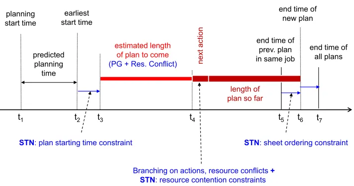
Figure 11: Important time points for constructing and evaluating a plan.
putting it after all other previous allocations by adding the temporal constraint en ≺ s.
However, there can also be gaps between the existing allocations [si, ei], allowing us to post
constraints such as ei ≺ s ≺ e ≺ si+1. Each such possible allocation for r generates a distinct child node in the search space. Because actionacan use several different resources r, the number of branches is potentially quite large. However, immediately resolving any potential overlaps in allocations for the same resource avoids the introduction of disjunctions in the temporal network, maintaining the tractability of temporal constraint propagation.
In summary, at every branch in the planner’s search space, we modify the logical state by branching over relevant actions and potentially introduce different temporal constraints in order to resolve resource contention. Because each branch results in a different irrevocable choice that is reflected in the final plan, the state at each node in the planner’s search tree is unique. Therefore, we do not need to consider the problem of duplicating search effort due to reaching the same state by two different search paths.
4.3.4 Heuristic Estimation
For each potential plan suffix, a lower bound is computed on the remaining makespan, in order to guide the planner’s A* search. Figure 11 illustrates how this heuristic estimate is used. In the figure, planning start time (t1) refers to the wall-clock time at which the planning process started andearliest-start-time = current wall-clock time + predicted
plan-ning time (t2) is the estimated time at which we will find a plan for the current sheet and
after the hypothetical plan starting time (t3+D ≺ t4) where D is the heuristic value on the makespan of the remaining plan to complete the current regressed partial-plan.
Our overall objective is to minimize the earliest possible end time ofall plans, including the sheet that we are planning for. This is indicated by the lower-bound on the floating time pointt7 in Figure 11. This time point is constrained to be after the end time points of all the sheets that have been planned and the one currently being planned. For the current sheet, this is represented by the constraints t6 ≺ t7 as shown in Figure 11. Because t6 is constrained to end after the completion time of all the other planned sheets in the same print job, the constraint essentially pushes t7 to be after all the sheets in the current print job end. To support this objective function, the primary criterion evaluating the promise of a partial plan (step 8 in Figure 6) is the estimate of the earliest possible happening time for t7, indicated by the STN embedded in this search node, after all constraints shown in Figure 11 are added in the current branch.
The key duration that affects t7 is the heuristic estimate of the lower bound on the additional makespan required to complete the current regressed plan. This heuristic value is indicated in Figure 11 byestimated remaining makespanbetweent3andt4. By adding the constraintt2≺t3, the insertion may thus change the earliest time of all the subsequent time pointst4,t5,t6 andt7. It may also introduce an inconsistency in the temporal database, in which case we can safely abandon the plan. Given that the current plan should end after the end time of all previous sheets in the same print job (t5 ≺t6), our objective function is to minimize t7 without causing any inconsistency in the temporal database. We break ties in favor of:
• smallert6 (e.g., end time of the current print job)
• smaller predicted makespan (t6−t3)
• larger currently realized makespan (t6 −t4). This is analogous to breaking ties on f(n) in A* search with larger g(n), and thus encourages further extension of plans nearer to a goal.
The performance of our search-based planner heavily depends on the quality of the heuristic estimating the makespan-to-go. We estimateDby building the temporal planning graph with adjustment for both logical mutex and resource contentions. For the rest of this section, we will discuss the details of how D is computed. Overall, we want an effective planning heuristic that is:
• Admissible: because maintaining high plan quality (high productivity of the printer)
is an important criterion for our customer.
• Informed and easy to compute: because in most cases, we are only allowed a fraction
of a second to find a feasible plan. Any delay in finding a plan will delay plan start execution time and thus reduce the overall productivity.
level. Starting with the initial state at timet= 0, the graph is grown forward in time with actions being activated when all of their preconditions are satisfied and non-mutex. There are three types of mutual exclusion relations (fact-fact, fact-action, action-action) that are propagated during the graph building process. The graph expansion phase alternates with the plan extraction phase starting from the time point at which all the goals appear non-mutex in the graph.
In our graph expansion algorithm, for each action a and factf, we store the first times ta and tf at which a can optimistically occur or f can optimistically be achieved. They
correspond to the first times at whichaandf appear in the temporal planning graph. For mutex propagation, we also store the first time point at which each pair of factshf1, f2i can be achieved together and each pair of actionsha1, a2i can execute together. In the planning graph, those are the first time points that hf1, f2i and ha1, a2i become non-mutex. In our implementation, a fact-action mutex between fact f and action a is converted into action mutex hnoopf, ai, as we will discuss later.
1. To begin: ∀f, a, f1, f2, a1, a2 :ta=tf =thf1,f2i=tha1,a2i=∞.
2. LetI be the initial state: ∀f, f1, f2 ∈I :tf = 0, thf1,f2i= 0.
3. Dynamically update the values of ta, tf, thf1,f2i, tha1,a2i starting from the initial state
I and time t= 0 as follows:
ta= max (setup time(a), max
f∈P rec(a)tf,f1,f2max∈P rec(a)
thf1,f2i) (1)
tf = min
f∈Eff(a)(ta+dur(a)) (2)
thf1,f2i = min (tha1,a2i+ max
f1∈Eff(a1),f2∈Eff(a2)
(dur(a1), dur(a2))) (3)
tha1,a2i= max (ta1, ta2, max
f1∈P rec(a1),f2∈P rec(a2)
thf1,f2i) (4)
The updates are done in the increasing order of time, as usual for planning-graph building algorithms.
4. Stop when ∀g∈G:tg<∞ and∀g1, g2 ∈G:thg1,g2i<∞ or we reach a fixed point.
implementation, we build the graph starting fromt= 0 by putting in events of (1) activating an action (updatingta); (2) activating a fact (updatingtf); and (3) removing a fact mutex
(updatingthf1,f2i), ordered by the time they occur. Each event will trigger new events to
happen at a later time. For example, adding a new factf or removing a fact mutexhf1, f2i can activate actions supported byf or by bothf1 and f2, and activating action awill add events of activating facts in Effect(a) and/or removing fact mutexes between Effect(a) and ‘noop’ (facts) that are not mutex with P recond(a). We also only explicitly store the fact-fact mutex timing values thf1,f2i but none of the action mutexes tha1,a2i, instead reasoning about them on-the-fly.
The time at which all the goals are achieved pair-wise non-mutex is the heuristic value estimating the remaining makespan to achieve the goal state (see Figure 11). While most regression planners (Haslum & Geffner, 2001; Nguyen, Kambhampati, & Nigenda, 2002) compute their heuristic once (until a fixed point is reached) before the planning process begins, in our case, the planning graph expansion process may be revisited if goals repre-senting a regressed state do not appear non-mutex in the graph and a fixed point was not reached in the previous round of expansion. Because only pair-wise mutexes are taken into account while building the graph, the estimated value is an underestimate of the makespan of any plan that can achieve the goal. Therefore, the returned value by the planning graph will lead to a underestimate (admissible heuristic) for both our objective function (overall end time t7) and tie breakers (current sheet end time t6 and current estimated makespan t6−t3) as described above. Therefore, using this estimate, the planner will return plan p with an optimal end time (minimum t7) and p also has a minimum makespan among all plans with the same end time.
Incorporating resource mutexes The planning graph discussed until now assumes
that the printer is empty. Thus, we create the planning graph similar to the procedure used in an off-line planner in which we assume the interference relations only occur between actions related to a given sheet that we are planning for. If the machine is empty, the heuristic is generally correct for simple sheets such as simplex printing and nearly correct for complicated sheets such as duplex printing.
However, most of the time, the printer is not empty and there are plans for sheets that are either (1) executing; or (2) found by the planner but haven’t been sent to the machine controller yet. Those plans involve resource allocations, either at fixed time points (for (1)) or at still flexible ones (for (2)). To find a more effective heuristic in those scenarios where the machine is busy, we take into account resource mutexes, thus incorporating scheduling resource contention constraints into the temporal planning graph. Figure 12 shows the pseudo-code of the algorithm. The key observation is that, to find the earliest time ta at
which an action a can possibly execute, a necessary condition is not only that all of a’s preconditions appear non-mutex in the planning graph but also that there is no resource conflict between any resourcer used byaand all current allocations ofr (given to previous plans and by external processes.)
As shown in the example action description in Figure 8, each resource allocation of action a is represented as a triple hr, o, di. If a starts at sa, this means that resource
r is used from sa +o for a duration d, which is normally different from the duration
Fig-1. Resource types: r1, r2, ....rn
2. All resource allocations: {R1, R2, ....Rn}
withRi ={[si1, ei1],[si2, ei2], ...[sim, eim]} the ordered list of allocations for ri
FunctionCheckEarliest(r, t, d) 3. r: resource
4. t: earliest time intend to user 5. d: duration intend to user
6. R={[s1, e1],[s2, e2], ...[sm, em]}: current allocations for r.
7. tmin: earliest time of a non-conflict allocation forr; initialize to: tmin←t
8. for each allocation l= [sk, ek]∈R check
9. if we can reserve r for a duration of dbeforelstarts: Latest(sk)> tmin+d
10. then go to line 14
11. else move forward to the next possible opening at the end of allocation a 12. tmin ←Earliest(ek)
13. end for; 14. return(tmin) end function;
Building the temporal planning graph
15. when consider adding action a to the planning graph
16. Initialize ta to the earliest time at which P rec(a) achieved non-mutex (eq.1)
17. Resource allocations of a: Ra={hr1, o1, d1i,hr2, o2, d2i, ...,hrn, on, dni}
18. for each allocation l=hrk, ok, dki check the earliest non-conflict time forl
19. ta←CheckEarliest(ri, ta+oi, di)−oi
20. end for;
21. add action ato the temporal planning graph at ta until all
goals appear non pairwise mutex;
Figure 12: Building the temporal planning graph with adjustments for resource conflicts.
ure 8 is (M arkingEngine,5.9,3.7). Lines 17-19 in Figure 12 show that when building the graph, for each action athat has all of its preconditions satisfied at ta, the algorithm goes
through all resources used by a. For each resource allocation hr, o, di, it calls the function CheckEarliest(r, ta+o, d) to updateta, the earliest executable time thatacan start without
overlapping with any of the previous resource allocations ofr. The pseudo-code of function CheckEarliest(r, t, d) is self-explanatory in that we try to find the earliest time point after tat which we can ‘slot’ the allocation forrwith duration din without overlapping with the previous allocations ofr.
Figure 13 shows one example to demonstrate this algorithm. In this example, we try to find the starting time for action a, which needs two unit-capacity resource allocations
t
1r
1r
2o
1t
2t
3d
1d
2o
2t
4t
5(1) (2) (3) (4)
(1) (2) (3) (4)
o
1A
:
s
Ae
Ar
1d
1r
2o
2d
2d
AFigure 13: Example of action starting time adjustment using resource contentions
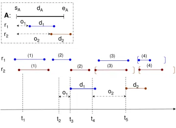
(2). The flexible allocations, shown with their upper/lower bound constraints are (4) for r1 and (3) and (4) forr2. Starting fromt1, the first time point at which we can allocater1 for a duration d1 without overlapping with previous allocations, both fixed and flexible, is t3. Thus, we adjust the new earliest possible starting time foratot2 =t3−o1≻t1. Given the new earliest possible starting time ta =t2, we find that the earliest time point from t2 at which we can allocate resource for r2 is t5. Given thatt4 =t5−o2 ≻t2, we will then take t4 as the final earliest starting time fora and activate action aat t4 in the graph (instead of the original valuet1)2.
With resource mutexes, the starting times of actions are adjusted to higher than the time points at which their preconditions can be achieved, and thus the time point tG at which
all the goals appear non-mutex in the graph is not an underestimation on the makespan of the remaining plan (valuet4−t3 in Figure 11). Thus,tGcan be higher than the summation
of the durations of actions in the optimal (serial) plan. However, tG still underestimates
the first time that we can achieve the goals and thus is still an admissible heuristic for our main objective function of minimizing the end time of current printing sheets (minimizing t7 in Figure 11). However, if we do not use the resource mutexes, then both the heuristic estimate for end time (t7) and the tie-breaker on plan makespan (t6 −t3) are admissible while with resource mutexes, only the estimate oft7 is admissible and the tie-breakert6−t3
0 0.5 1 1.5 2
1 4 7 10 13 16 19 22 25 28 31 34 37 40 43 46 49
ti
m
e
(
s
e
c
) no-mutexlogical mutex log + res mutex productivity level
Figure 14: Performance for the prototype built by our industrial partner.
can be inadmissible. Thus, the A* algorithm is still guaranteed to find an optimal solution, minimizing the plan end-time, but the final solution will not be guaranteed to have a shortest duration among all plans that finish earliest.
4.4 Evaluation of Nominal Planning
0.01 0.1 1 10
1 6 11 16 21 26 31 36 41 46
jobs
ti
m
e
(
s
e
c
)
nomutex logical mutex log + res mutex productivity level
Figure 15: Performance for the current prototype built by us and shown in Figure 1. Note that time is plotted logarithmically.
Figure 14 and 15 show the performance of our planner in two of the most complex parallel printer prototypes built by Xerox and by us. Their productivity levels are higher than any other printer of the same class currently on the market. In each figure, we show the CPU time consumed per-sheet for the basic test of using the planner for a print job of 50 sheets: (1) without mutexes; (2) with serial temporal planning graph with mutexes; (3) combination of logical and resource mutexes; and (4) the baseline requirement for the planner’s performance to match with the printer’s full productivity. The other prototypes investigated using our planner are either simpler or more complicated but used for the-oretical investigations only. For the rest of this section, we will refer to the first printer (results shown in Figure 14) asConfiguration 1 and the other (results shown in Figure 15)
asConfiguration 2.
The Configuration 1 printer in Figure 14 is the simpler one, with 25 main components
The Configuration 2 printer tested in Figure 15 is the more complicated one. There are 212 action schemata and the shortest possible plan contains 16 actions. The printer generally handles more than 20 sheets at a time so the planner needs to regularly reason about the interactions between more than 300-400 actions. The productivity level of this printer is 220 pages-per-minute, which leads to the base running time for the planner of 60/220 = 0.27 second for planning a single sheet. Because of the wider gap in performance between different versions of the planners, we show timing results for this printer in log scale. Without using mutexes, the planner quickly overruns the time limit after a few sheets and grows to more than 10 seconds around sheet 35, when we stopped the experiment. With mutexes (logical, resource) the planner generally takes less than 0.3 second to find a plan. However, occasionally the planner takes longer. But because it usually plans ahead around 10 sheets before releasing plans to the lower level controller, occasional jumps in planning time don’t prevent the planner from achieving the full productivity of the printer in practice. The planner averages 0.1336 second with only logical mutexes and 0.0928 second (1.44x improvement) if used in conjunction with resource mutexes.
The results in Figure 14 and 15 indicate that the average planning time for individual sheets increases with the number of previous sheets. This is due to the fact that the planner generally plans faster than the speed at which the printer can print. Thus, as the number of print requests received increases, the number of plans in theunsent queue (i.e., planned for, but not sent to the machine yet) increases. This increases the resource contention and branching factor when searching for a new plan, which leads to the increment in planning time. Eventually, the number of lookahead sheets reaches a point where the planning time equals the planner’s productivity and a dynamic equilibrium is reached. The planning time does not strictly increase linearly in accordance with the number of sheets planned, but rather shows an oscillating pattern. This is due to the complex interaction between the on-line processes of planning, freezing time points in the found plan, and plan execution. This can lead to easier planning problems when there are more sheets, depending on how those sheets interact with the sheet that is currently being planned.
While it was noted by Smith and Weld (1999) and other work based on building the planning graph that mutex propagation is costly, this was not our experience. In fact, when the printer is rather empty, the total planning time, which subsumes the graph with mutex building time is less than 0.01 second. We believe that this is due to a simpler mutex propagation rule in our planner and the fact that the sequential plan of each sheet makes all actions mutex at each step. Our resource mutex reasoning time is not as optimized as the logical mutex implementation and can be improved, but it does not seem to be a significant impediment in our intended application.
LPG SGPlan Hybrid
# Span Time Span Time Span Time
1 9.3 0.01 8.3 0.45 8.3 <0.001
2 13.3 0.02 9.3 308.46 9.4 <0.001
3 26.6 0.08 - - 9.9 0.02
4 15.2 0.07 - - 10.6 0.02
5 21.3 0.12 - - 11.1 0.03
6 22.4 0.23 - - 11.8 0.03
7 30.3 8.73 - - 12.3 0.04
8 19.6 52.55 - - 13.0 0.06
9 24.2 16.69 - - 13.5 0.07
10 23.0 20.02 - - 14.2 0.07
11 29.7 40.14 - - 14.7 0.08
12 18.3 138.53 - - 15.4 0.09
13 42.6 29.09 - - 15.9 0.18
14 34.9 427.41 - - 16.6 0.21
15 35.3 18.95 - - 17.1 0.28
Table 1: Comparison of LPG, SGPlan, and our hybrid planner, showing the makespan of the plans found (‘Span’) and planning times (‘Time’) in seconds for problems with various numbers of sheets (‘#’).
4.4.1 Scaling Against Generic Planners
Although our planner has certain features, such as controllable action durations, that are beyond the capabilities of existing planners, it is still interesting to compare against off-line systems to validate our new approach. If existing generic systems could solve basic printing control problems well, it might be possible to extend them, rather than developing the more specialized planner architecture described above. Therefore, we built a tool to automatically convert our custom domain language into the PDDL2.1 temporal planning language, allowing us to test current state-of-the-art planners.