Rank Set Sampling in Improving the Estimates of Simple Regression Model

Simple Regression Model

M. Iqbal Jeelani

Division of Agricultural Statistics, SKUAST-K, India [email protected]

S.A. Mir

Division of Agricultural Statistics, SKUAST-K, India [email protected]

I. Khan

Division of Agricultural Statistics, SKUAST-K, India [email protected]

S.Maqbool

Division of Agricultural Statistics, SKUAST-K, India [email protected]

Nageena Nazir

Division of Agricultural Statistics, SKUAST-K, India [email protected]

Fehim Jeelani

Division of Agricultural Statistics, SKUAST-K, India [email protected]

Abstract

In this paper Rank set sampling (RSS) is introduced with a view of increasing the efficiency of estimates of Simple regression model. Regression model is considered with respect to samples taken from sampling techniques like Simple random sampling (SRS), Systematic sampling (SYS) and Rank set sampling (RSS). It is found that R2 _{and Adj R}2 _{obtained from regression model based on Rank set sample is higher than rest}

of two sampling schemes. Similarly Root mean square error, p-values, coefficient of variation are much lower in Rank set based regression model, also under validation technique (Jackknifing) there is consistency in the measure of R2_{, Adj R}2 _{and RMSE in case of RSS as compared to SRS and SYS. Results}

are supported with an empirical study involving a real data set generated of Pinus Wallichiana taken from block Langate of district Kupwara.

Keywords: Rank set sampling, Simple Regression Model, Pinus Wallichiana. 1. Introduction

part of this process is laboratory analysis, while identification of potential sample units is comparatively simple. We can therefore achieve great observational economy if we are able to identify a large number of sample units to represent the population of interest, yet only have to quantify a carefully selected subsample. This potential for observational economy was recognized for estimating mean pasture and forage yields in the early 1950s, when McIntyre (1952) proposed a method, later coined Rank set sampling (RSS) by Halls and Dell (1966). McIntyre (1952) developed the procedure of RSS to find a more efficient method to estimate the yield of pastures. Measuring yield of pasture plots requires mowing and weighing the hay which is time-consuming. However experience can be used to rank by eye inspection to a large extent accurately the yields of a small number of plots without actual measurement. McIntyre (1952) adopted the sampling scheme, where, each time a random sample of k pasture lots is taken and the lots are ranked by eye inspection with respect to the amount of yield from the first sample, the lot with rank 1 is taken for cutting and weighing. From the second sample, the lot with rank 2 is taken, and so on. When each of the ranks from 1 to k has an associated lot being taken for cutting and weighing, the cycle repeats over again and again until a total of m cycles are completed. McIntyre (1952) observed that the relative efficiency, defined as the ratio of the variance of the mean of a simple random sample and the variance of the mean of a ranked set sample of the same size, is not much less than (k+1)/2 for symmetric or moderately asymmetric distributions, and that the relative efficiency diminishes with increasing asymmetry of the underlying distribution but is always greater than 1. He observed that by using the same sample size RSS provides an increased precision as compared to simple random sampling (SRS).

schemes for handling Non-Response problems in Rank set sampling under stratification has been suggested by Jeelani et al (2014,b).

In this paper data on Pinus Wallichiana is utilized. The data on Pinus Wallichiana was taken from block Langate of District Kupwara from Forest department J&K. Pinus Wallichiana is a coniferous evergreen tree native to the Himalaya, Karakoram and Hindu Kush mountains, from eastern Afghanistan east across northern Pakistan and India to Yunnan in southwest China. It grows in mountain valleys at altitudes of 1800–4300 m (rarely as low as 1200 m), between 30 m and 50 m in height. It favours a temperate climate with dry winters and wet summers. This tree is often known as 'Bhutan pine', (not to be confused with the recently described Bhutan white pine, Pinus bhutanica, a closely related species). Other names include 'blue pine', 'Himalayan white pine' and 'Himalayan blue pine'. In the past, it was also known by the invalid botanic names Pinus griffithii McClelland or "Pinus excelsa" Wall., Pinus chylla Lodd. when the tree became available through the European nursery trade in 1836, nine years after Dr Wallich first introduced seeds to England. The leaves ("needles") are in fascicles (bundles) of five and are 12–18 cm long. They are noted for being flexible along their length, and often droop gracefully. The cones are long and slender, 16–32 cm, yellow-buff when mature, with thin scales; the seeds are 5–6 mm long with a 20–30 mm wing. Typical habitats are mountain screes and glacier forelands, but it will also form old growth forests as the primary species or in mixed forests with deodar, birch, spruce, and fir. In some places it reaches the tree line. The wood is moderately hard, durable and highly resinous. It is a good firewood but gives off a pungent resinous smoke. It is a commercial source of turpentine which is superior quality than that of P. roxburghii but is not produced so freely. It is also a popular tree for planting in parks and large gardens, grown for its attractive foliage and large, decorative cones. It is also valued for its relatively high resistance to air pollution, tolerating this better than some other conifers.

2. Material Methods

In this paper simple linear regression model is considered with respect to samples taken from the sampling techniques like simple random sampling (SRS), systematic sampling (SYS) including rank set sampling (RSS).The method of estimation used in this paper is the ordinary least squares method (OLS). Also, bivariate ranked set sample is introduced, Al-Saleh and Zheng (2002). Finally regression models based on different identified sampling schemes are compared with each other based on validation technique (Jackknifing), which is a sample reuse technique, Quenouille (1949). A bivariate rank set sampling given by Al-Saleh and Zheng (2002) can be obtained as follows:

Suppose (X, Y) is a bivariate random vector with the joint probability density function (jpdf) f (x, y).

1. A random sample of size k4 _{is identified from the population and randomly}

2. In the first pool, identify by judgment the minimum value w.r.t. the first characteristic, for each of the k rows.

3. For the k minima obtained in Step 2, choose the pair that corresponds to the minimum value of the second characteristic, identified by judgment, for actual quantification. This pair, which resembles the label (1, 1), is the first element of the bivariate rank set sample.

4. Repeat Steps 2 and 3 for the second pool, but in step 3, the pair that corresponds to the second minimum value w.r.t the second characteristic is chosen for actual quantification. This pair resembled the label (1, 2).

5. The process continues until the label (k, k) is resembled from the (k2)th (last) pool. The above procedure produces a Bivariate rank set sample of size k2_{. Thus we}

have k2 observations denote by: (X[i](j) ,Y(i)[j]), i=1,2…k and j=1,2,…k.

6. The procedure can be repeated m times to obtain a sample of size n = k2m which will be denoted by (X[i](j)k, Y(i)[j]k), i=1,2…k and j=1,2,…k, k=1,2,m.

In this article, effect of BVRSS on simple regression model is investigated utilizing Y and X as random variables. An important feature of BVRSS is that ranking is done on both variables Y and X simultaneously. Inference for simple regression model parameters (𝛼 , 𝛽) using asymptotic results are given. The simple regression model of the two variables Y and X is defined by: y_(i)[j]t  a  X_[i](j)t  E_ijt where a is the model intercept, β is the model slope and Eijt is the random error. The assumptions needed here for the purpose of parameters estimation are the mean of the error is zero, its variance is finite and they uncorrelated. Also Xi and Ei are independent. Then the least squares estimators of a and β are given by:

bvrss bvrss bvrss

bvrss Y  X

    (2.1)

bvrss i j t bvrss kt j i bvrss t j i i j t bvrss t j i bvrss X X X Y y X X ) ) ( ( ) ( . . 2 ) ]( [ . ] )[ ( . . ) ]( [





 (2.2)

where and . . ) ]( [ n X X tji

t j i bvrss



t j i bvrss



Y     2[]( )

2 t j i X    (2.4)

Then the fitted model is

t j i bvrss bvrss t j

i a X

Y_{()[ ]}   _{[]( )}

(2.5) t j i t j i t j i t j

i Y Y

e_{()[ ]} _{()[ ]}  _{()[ ]}  _{[]( )}

Also, a consistent unbiased estimator for     



t j i e e . . 2 ] )[ ( 2 2  (2.7)

where  is number of parameters to be estimated in simple regression model Assuming the conditions of the regression model above, then



 

 ( )

)

(a_bvrss aE _bvrss

E  

(2.8) )] ( 1 [ ) ( ₂ , 2 2 bvrss X bvrss e bvrss S X E n a

Var   

(2.9) where n X X

S t ji

bvrss t j i bvrss X



Var   

(2.11) t j i i i t j

i X x a x

Y

E(_{()[ ]} /  )  _{()[ ]} (2.12)

)] ) ( ( 1 [ ) ( 2 , 2 ) ]( [ 2 ] )[ ( bvrss X bvrss t j i e t j i S X x E n Y

Var     2()[ ]

2 t j i X    (2.13) 0 ) (e_(i)[j]t  E (2.14) )] ) ( ( 1 [ 1 [ ) ( ₂ , 2 ] )[ ( 2 ] )[ ( bvrss X bvrss t j i e t j i nS X x E n e

Var     (2.15)

)] ) ( ( ) , ( cov 2 2 bvrss bvrss e bvrss bvrss Y X E n

a    (2.16)

2 2

)

( _{e e}

E  (2.17)

     n Var e e 4 2 2 )

( (2.18)

where  is number of parameters to be estimated in simple regression model

2 2

e e 

  (2.19)

)] ) (

1 [

) (

1 [ ( ) , ( efficiency

2 , 2 2 , 2

bvrss X

bvrss bvh X

bvh

bvh bvrss

S X E

S X E

a

  

 

(2.20)

Where bvh = bvsrs, bvsys

)] 1

1 (

) , ( efficiency and

2 ,

2

bvrss X

bvh bvh

bvrss

S E

S E





  (2.22)

where;

𝐸(𝑌) = 𝜇𝑦 , 𝑣𝑎𝑟(𝑌) = 𝜎𝑦2 , 𝐸(𝑋) = 𝜇𝑥 , 𝑣𝑎𝑟(𝑋) = 𝜎𝑥2 , 𝑣𝑎𝑟(𝑌) = 𝜎𝑦2, 𝜌 =

𝑐𝑜𝑣(𝑌, 𝑋) 𝜎⁄ _𝑦𝜎_𝑥, 𝐸(𝑋[𝑖](𝑗)) = 𝜇𝑋[𝑖](𝑗), 𝐸(𝑌(𝑖)[𝑗])) = 𝜇𝑌(𝑖)[𝑗] , 𝐸(𝑋[𝑖](𝑗)2 ) = 𝜇𝑋[𝑖](𝑗)(2) ,

𝐸(𝑌_(𝑖)[𝑗]2 ) = 𝜇_{𝑌(𝑖)[𝑗]}(2) , 𝑣𝑎𝑟(𝑋_[𝑖](𝑗)) = 𝜎_{𝑋[𝑖](𝑗)}(2) , 𝑣𝑎𝑟(𝑌_(𝑖)[𝑗]) = 𝜎_{𝑌(𝑖)[𝑗]}(2) , 𝑐𝑜𝑣( 𝑋_[𝑖](𝑗), 𝑌_(𝑖)[𝑗]= 𝜎_{(𝑋[𝑖](𝑗),𝑌(𝑖)[𝑗]}

3. Numerical illustration

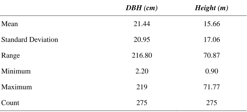
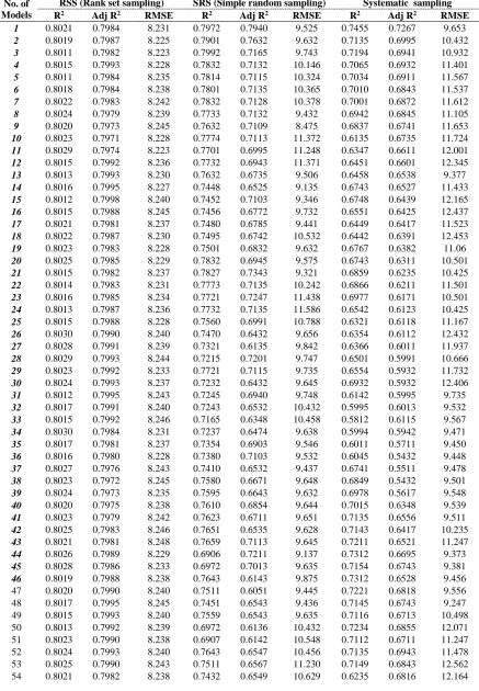
Assume that (X, Y) follow a bivariate normal distribution, the performance of simple regression model using BVSRS, BVSYS and BVRSS was judged with the help of a data set. The original data was collected on two variables of Pinus Wallichiana: where, “X” is the diameter in centimeters at breast height and “Y” is the entire height in feets. The regression model is analyzed assuming that the population consists of 275 trees. The summary statistics of the data is reported in Table-1. A sample size of 55 was fixed in all the sampling designs to make comparisons. Regression analysis and regression diagnostics in all the three sampling designs was carried out in SAS software using the function POC REG. The layout of RSS is given in Table-2. The relative efficiency of RSS with SRS and SYS along with R2 and Adj R2 are given the Table-3. The performance of RSS with SRS and SYS is also judged with the help of validation technique i.e. Jack-knifing carried out in SAS using function PROC JACKREG in Tables-5 to 7.

4. Conclusion

Systematic Sampling. The above results occurred because rank set samples are more regularly spaced than those obtained from Simple Random Sampling and Systematic Sampling and therefore more representative of the population. Because of Ranking the Rank Set Sampling procedure induces stratification at sample level which involves the gained precision in this scheme. Obtaining a sample in this manner maintains the un-biasedness of simple random sampling; however, by incorporating outside information about the sample units, we are able to contribute a structure to the sample that increases its representativeness of the true underlying population. If we quantified the same number of sample units, by a simple random sample or a systematic sample then we have no control over which units enter the sample. Perhaps all the units would come from the lower end of the range, or perhaps most would be clustered at the low end while one or two units would come from the middle or upper range. With other sampling techniques, the only way to increase the prospect of covering the full range of possible values is to increase the sample size. Rank set sampling has a balanced nature in the sense that equal number of observations will be obtained from each rank. It can be easily shown that the sample mean using Rank set sampling has a smaller variances than its counter parts when the number of observations are the same.

Acknowledgment

The first author wishes to record his gratitude and thanks to University Grants Commission, Govt. of India, for providing the UGC National Fellowship for perusing the Doctorate prorgramme in Statistics. Also the authors would like to thank Mr. Irfan Rasool (IFS) DFO, District Kupwara for providing the data for the preparation the manuscript.

References

1. Al-Saleh, M.F. and Zhengh, G. (2002). Estimation of Bivariate characteristics using rank set sampling. Australian and New Zealand Journal of Statistics., 44(1), 221-232.

2. Cobby, J.M., Ridout, M.S., Bassett, P.J. and Large, R.V. (1985). An investigation into the use of ranked set sampling on grass and grass-clover sward. Grass and Forage Science 40: 257-263.

3. Cochran, W.G. (1977). Sampling Techniques. John Wiley and Sons, New York. 4. Dell, T.R. and Clutter, J.L. 1972. Ranked set sampling theory with order statistics

background. Biometrika. 28: 545-555.

5. Dell, T.R. and Clutter, V. (1972). Ranked set sampling theory with order statistics background. Biometrics 28: 545-555.

6. Gaajendra, K.A. and Bouza, C. (2012). Double sampling with rank set selection in the second phase with non-response: Analytical results and Monte carlo experiments. Journal of Probability and Statistics 23: 45-53.

8. Jeelani, M.I., Mir, S.A., Maqbool, S., Khan, I., Singh, K.N., Zaffer, G., Nazir, N. and Jeelani, F. (2014). Role of Rank Set Sampling in Improving the Estimates of Population Mean under Stratification. Amer. J. Math. and Statist., 4(1), 46-49.

9. Kamarulzaman, I. (2011). On comparison of some variation of rank set sampling.

Sains Malaysiana 40: 397-401.

10. Martin, W.L., Shank, T.L., Oderwald, R.G. and Smith, D.W. (1980). Evaluation of ranked set sampling for estimating shrub phytomass in Appalachian Oak forest. Technical Report No.FWS-4-80, School of Forestry and Wildlife Resources VPI & SU Blacksburg, VA.

11. McIntyre, G. A. (1952). A method for unbiased selective sampling using ranked sets. Australian Journal of Agricultural Research 3: 385-390.

12. McIntyre, G. A. (1978). Statistical aspects of vegetation sampling: Measurement of Grassland Vegetation and Animal Production. Commonwealth Bureau of Pastures and Field Crops. Hurley, Berkshire, UK. 45: 8-21.

13. Nussbaum, B.D. and Sinha, B.K. (1997). Cost effective gasoline sampling using ranked set sampling. In a Proceedings of the Section on Statistics and the Environment. American Statistical Association 41:

14. Quenouille, M.H. 1956. Notes on bias in estimation. Biometrik, 43: 353-360.

15. Samawi, H.M and Abu-Dayyeh, W. (1997). Estimating the population mean using bivariate rank set sampling, Biometrical Journal., 38 (5), 577-586.

16. You, G. (2009). Efficient designs for sampling and sub sampling in fisheries research based on ranked sets. Journal of Marine Science.66: 928-934.

Table 1: Summary statistics of the Pinus data

DBH (cm) Height (m)

Mean 21.44 15.66

Standard Deviation 20.95 17.06

Range 216.80 70.87

Minimum 2.20 0.90

Maximum 219 71.77

Table 2: Layout of RSS based on ranking (dbh ‘cm’ and height ‘feets’) simultaneously

Cy

cles

Set size = k= 5 ( N= 275, n = 55, means we have to repeat the process of ranking (m=11) 11 times i.e. 11×5 = 55

Tree Number 1 2 3 4 5

Height 15.9 22 56.9 9.6 24.6

Cy

cle 1

(dbh) 28.0 26.0 119.0 16.0 43.0

Tree Number 6 7 8 9 10

Height 3.3 11.4 4.7 21.3 16.8

(dbh) 7.0 21.0 6.0 40.0 28.0

Tree Number 11 12 13 14 15

Height 5.1 7.5 3.1 4.9 6.1

(dbh) 12.0 22.0 7.0 7.0 9.0

Tree Number 16 17 18 19 20

Height 5.5 6.5 5.6 6.9 3.8

(dbh) 12.0 11.0 14.0 11.0 6.0

Tree Number 21 22 23 24 25

Height 9.7 6.9 4.1 58.5 46

(dbh) 27.0 16.0 8.0 192.0 203.0

Cy

cle 1

1

Tree Number 251 252 253 254 255

Height 10.9 3.5 2.5 10.9 8.9

(dbh) 33.0 6.0 4.0 26.0 24.0

Tree Number 256 257 258 259 260

Height 21 44.1 7.0 9.4 8

(dbh) 67.0 107.0 16.0 27.0 17.0

Tree Number 261 262 263 264 265

Height 23 11.6 33 7.5 17.5

(dbh) 59 35.0 90.0 17.0 46.0

Tree Number 266 267 268 269 270

Height 8.9 47.4 22 6.8 7.5

(dbh) 33.0 53.0 49.0 18.0 18.0

Tree Number 271 272 273 274 275

Height 22.2 19.3 14.5 3.5 10.9

(dbh) 32.0 25.0 22.0 5.0 26.0

For the sake of simplicity only 1st _{and 11}th _{cycle is presented here, where figures in} italics are tree numbers and figures in bold are dbh ‘cm’ and height ‘feets’

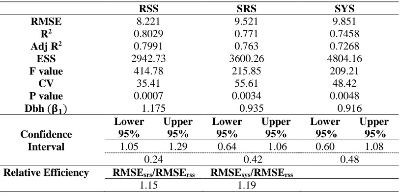
Table 4: Relative efficiency of RSS with SRS and SYS along with R2_{, Adj R}2 _and others measures of comparison

RSS SRS SYS

RMSE 8.221 9.521 9.851

R2 _{0.8029 0.771 0.7458}

Adj R2 _{0.7991 0.763 0.7268}

ESS 2942.73 3600.26 4804.16

F value 414.78 215.85 209.21

CV 35.41 55.61 48.42

P value 0.0007 0.0034 0.0048

Dbh (𝛃_𝟏) 1.175 0.935 0.916

Confidence Interval

Lower 95%

Upper 95%

Lower 95%

Upper 95%

Lower 95%

Upper 95% 1.05 1.29 0.64 1.06 0.60 1.08

0.24 0.42 0.48

Table 5: Comparison of regression models based on various schemes using Jack-knifing

No. of Models

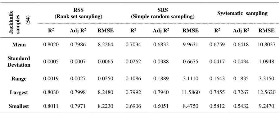
Table 6: Summary statistics of regression model based on sampling designs using Jacknifing

J

a

ck

k

n

ife

sa

m

p

les

(5

4

)

RSS (Rank set sampling)

SRS

(Simple random sampling) Systematic sampling R2 _{Adj R}2 _{RMSE R}2 _{Adj R}2 _{RMSE R}2 _{Adj R}2 _RMSE

Mean 0.8020 0.7986 8.2264 0.7034 0.6832 9.9631 0.6759 0.6418 10.8037

Standard

Deviation 0.0005 0.0007 0.0065 0.0262 0.0388 0.6675 0.0417 0.0434 1.0948 Range 0.0019 0.0027 0.0250 0.1086 0.1889 3.1110 0.1643 0.1835 3.3150

Largest 0.8030 0.7998 8.2480 0.7992 0.7940 11.5860 0.7455 0.7267 12.5620

Smallest 0.8011 0.7971 8.2230 0.6906 0.6051 8.4750 0.5812 0.5432 9.2470

*_{(Each observation is based on 54 jackknife samples)}

Table 7: Parameters of comparison of actual regression model

RSS (Rank set sampling) SRS (Simple random sampling) Systematic sampling

R2 _{Adj R}2 _{RMSE R}2 _{Adj R}2 _{RMSE R}2 _{Adj R}2 _RMSE